Background
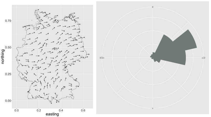
Circular data, i.e., data defined on the unit circle, can be found in many areas of science. The unique nature of these data means that conventional methods for non-circular data are not valid for these. At the same time, advances in geographical information and global positioning systems have generated large amounts of spatial data and, consequently, have increased the need for spatial models that accurately describe it. An example of circular, spatial data are the average wind directions in Germany from April 1 to 10, 2019, plotted in space (left) and on a circular histogram (right):
It was Jona-Lasinio, Gelfand, and Jona-Lasinio (2012) and Wang and Gelfand (2014) that first brought the wrapped and projected Gaussian distributions to space and space-time settings. Nonetheless, today,circular data models still need to catch up on the latest advances in spatial statistics. In particular, models developed so far assume stationarity in the mean and the covariance of the response modeled; i.e., these are constant in space. Our work in Marques, Kneib, and Klein (2022) aims to bridge this gap and allow for non-stationarity in the mean and covariance of distributions for circular responses defined on spatial domains.
The response distribution
To construct distributions for circular data, we can rely on the construction principle of wrapping the distribution of a random variable \(Y \in \mathbb{R}\) defined on the real line around the unit circle to make its domain adhere to the interval \([0,2\pi]\). The result is a circular – or wrapped – random variable \(X \in \lbrack 0,2\pi)\). Then, the unwrapped variable \(Y\) can be expressed as \[ Y = X + 2 \pi K \] where \(K \in \mathbb{Z}\) measures the number of “turns” \(Y\) has be wrapped around the unit circle.
Let \(\mathbf{s}\) denote a spatial index variable within a spatial domain \(S \subset \mathbb{R}^2\). Jona-Lasinio, Gelfand, and Jona-Lasinio (2012) first showed that this wrapping approach can be extended to the context of spatial data. We extend their framework and consider \[ X(\mathbf{s}_i) = \beta_0 + \mathbf{z}(\mathbf{s}_i)' \boldsymbol{\beta} +\gamma(\mathbf{s}_i, \mathbf{z}^\kappa(\mathbf{s}_i)) + 2 \pi K(\mathbf{s}_i) + \varepsilon_i ,\] where \(i=1, \ldots,n\), \(\gamma(\mathbf{s}_i)\) is a zero-mean Gaussian random field (GRF) and \(\varepsilon_i \sim N(0, \sigma^2_\varepsilon)\) are the i.i.d. error terms, with the following novelties:
The mean depends on \(\mathbf{z}(\mathbf{s}_i)' \boldsymbol{\beta}\), i.e. it is non-stationary,
The covariance depends on \(\mathbf{z}^\kappa(\mathbf{s}_i)\), i.e. it is non-stationary,
We include small-scale noise \(\varepsilon_i\)s.
We focus on 1. and 2.
1. Non-stationarity in the mean
Linear covariates included in the mean of a circular response might induce a circular likelihood for the regression coefficients that has infinitely many maxima. The typical solution is to use a link function for fixed effects with co-domain defined in \(\mathbb{R}\) and of length equal to the circular variable’s period of \(2\pi\), e.g. the inverse tangent link function.
We argue that:
The winding number \(K(\mathbf{s})\) can govern the behavior of the combination of GRF and fixed effects such that no link function is needed,
We use prior information that shrinks towards a stationary mean and enforces the length of the fixed effects to be approximately \(2\pi\).
Concretely, \(\beta_0 \sim N(0, 10)\) represents a diffuse prior for the intercept and we let \(\boldsymbol{\beta} \vert \xi^2 \sim N(\mathbf{0}, \xi^2 \mathbf{I})\). One can show that if the base model is such that \(\xi^2 \to 0\) and the prior is constructed according to the PC-prior principles (Simpson et al. 2017), then \(\xi^2\) has a Weibull prior with shape \(\frac{1}{2}\) and scale \(\lambda\), i.e., \(\xi^2 \sim \text{Weibull}(\frac{1}{2}, \lambda)\) (Klein and Kneib 2016).
For \(\alpha \in (0, 1)\), \(\lambda\) is chosen such that \[ P\left( \text{max}_{\mathbf{s} \in S} \mid \mathbf{z}(\mathbf{s})'\boldsymbol{\beta} \mid \leq\, \pi \right) \geq 1 - \alpha, \] i.e., the probability that the maximum norm of the non-stationary effect in the mean of the response is smaller than \(\pi\) is larger than \(1 - \alpha\). The value \(\pi\) in the expression is close to the recommendation of \(3\) in Klein and Kneib (2016).
2. Non-stationarity in the covariance
The stochastic partial differential equation (SPDE) approach (see Lindgren, Rue, and Lindström 2011) allows us to model non-stationarity in the covariance of the GRF in a computationally efficient way. Consider the parameters of the Matérn covariance with smoothness \(1\) and \(\kappa\) and \(\tau\) controlling the range and the marginal variance of the GRF, respectively.
We let \[ \log(\tau) = \theta^\tau_0 \mbox{ and } \log(\kappa(\mathbf{s})) = \theta^\kappa_0 + \mathbf{z}^\kappa(\mathbf{s})'\boldsymbol{\theta}^\kappa_z, \] where uniform priors for \(\theta^\tau_0\) and \(\theta_0^\kappa\) guarantee that the marginal variance is in \([0.01, (2\pi)^2]\) and the spatial range is in \([0.01, 1]\) for \(S \subseteq [0, 1] \times [0,1]\). Once again, we use a simulation-based method to guarantee
\[ P\left( \text{max}_{\mathbf{s} \in S} \mid \mathbf{z}^\kappa(\mathbf{s})'\boldsymbol{\theta}^\kappa_z \mid \leq\, c \right) \geq 1 - \alpha_\kappa, \] such that \(c\) guarantees that the spatial range satisfies \(\rho(\mathbf{s}) \in [0.01, 1]\), with typically \(c = 3\) (see Klein and Kneib 2016). The resulting prior structure shrinks towards a model with stationary covariance.
More concretely, we have \(\theta^\tau_0 \sim U(-10, 3)\), \(\theta^\kappa_0 \sim U(1, 6)\) and \(\boldsymbol{\theta}_z^\kappa \vert \zeta^2 \sim N(\mathbf{0}, \zeta^2 \mathbf{I})\), with \(\zeta^2 \sim \text{Weibull}(\frac{1}{2}, \lambda_\kappa)\).
The full-hierarchical model
The SPDE is typically used in combination with integrated nested Laplace approximations (INLA). However, INLA does not perform well when combined with shrinkage priors for non-stationarity in the covariance as defined here. Thus, we use Markov Chain Monte Carlo with full-hierarchical model:
\[\begin{align*} X(\mathbf{s}) &= \eta(\mathbf{s}) + 2 \pi K(\mathbf{s}) + \varepsilon, \\ &= \beta_0 + \mathbf{z}(\mathbf{s})' \boldsymbol{\beta} + \gamma(\mathbf{s}, \mathbf{z}^\kappa(\mathbf{s})) + 2 \pi K(\mathbf{s}) + \varepsilon,\\ \beta_0 &\sim N(0, 10) ,\mbox{ } \boldsymbol{\beta} \vert \xi^2 \sim N(0, \xi^2 \mathbf{I}), \mbox{ }\boldsymbol{\gamma} \vert \boldsymbol{\theta} \sim N(\mathbf{0}, \mathbf{Q}^{-1}(\boldsymbol{\theta})) \\ \theta_0^\tau &\sim U(-10, 3) ,\mbox{ } \theta_0^\kappa \sim U(1, 6) ,\mbox{ } \boldsymbol{\theta}^\kappa_z \vert \zeta^2 \sim N(\mathbf{0}, \zeta^2 \mathbf{I}) \\ \xi^2 &\sim PC\left(\pi, \alpha \right) ,\mbox{ } \zeta^2 \sim PC\left(3, \alpha_\kappa \right) \\ \mathbf{\varepsilon} \vert \sigma^2_\varepsilon &\sim N(\mathbf{0}, \sigma^2_\varepsilon \mathbf{I}) ,\mbox{ } \sigma^2_\varepsilon \sim IG (0.001, 0.001)\\ p(K(\mathbf{s})) &= \begin{cases} \frac{1}{3},& \text{if } K(\mathbf{s}) \in \lbrace -1, 0, 1 \rbrace\\ 0, & \text{otherwise} \end{cases} \end{align*}\]
Outcome
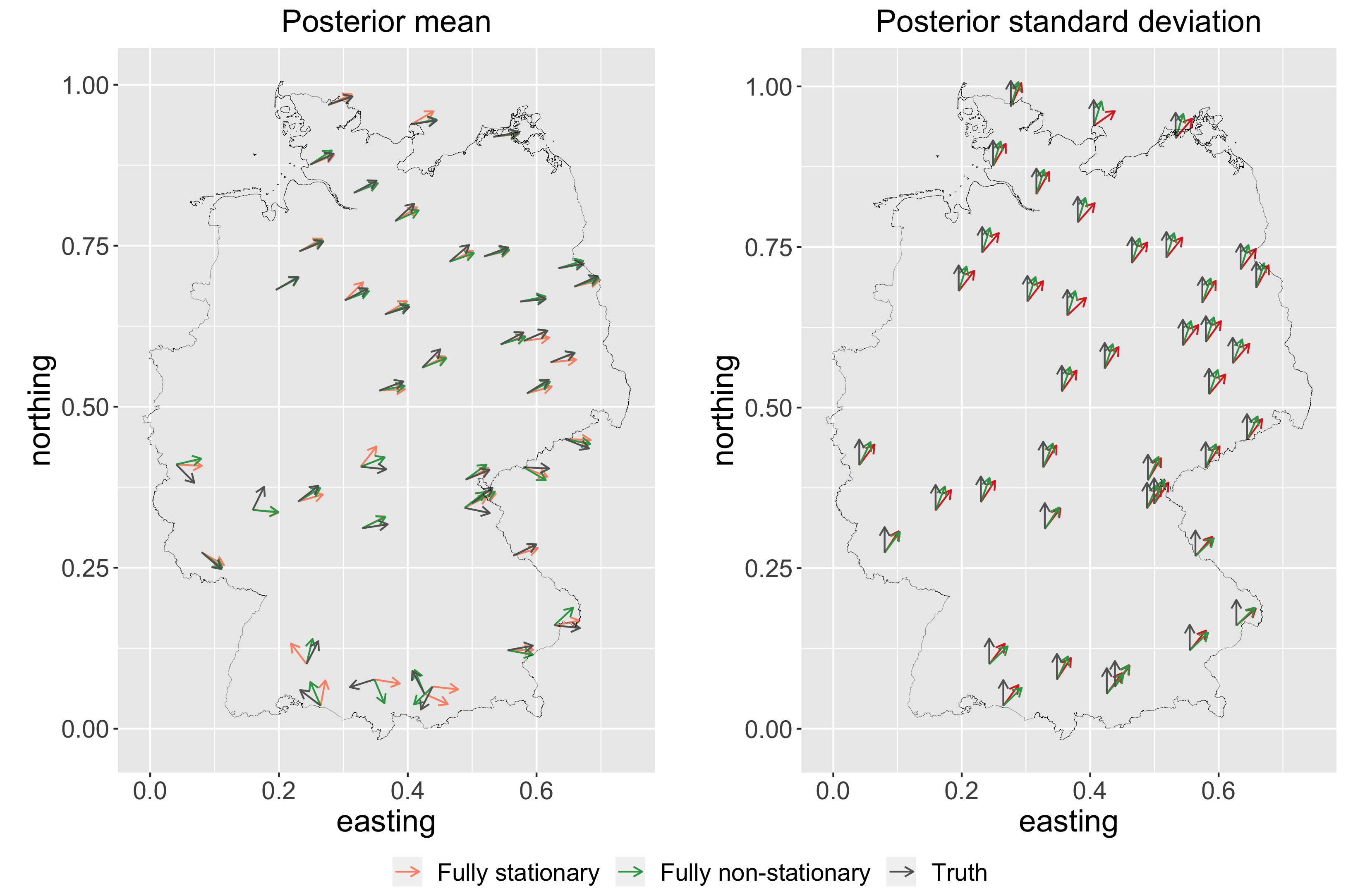
One can use our model to estimate wind directions in the dataset above and test the model’s performance. We randomly select a holdout set consisting of \(20\%\) of the locations and use the remaining \(80\%\) as training data. The covariates considered for \(\mathbf{z}(\mathbf{s})\) are maximum wind speed, average air humidity, and temperature at 10 meters height. For \(\mathbf{z^\kappa}(\mathbf{s})\) we consider altitude and latitude.
The figure below shows the posterior predictive mean (left) and standard deviation (right) for each test location for a fully stationary, i.e., stationary mean and covariance and fully non-stationary models. The black arrows represent the true wind directions (left) and the corresponding standard deviation of zero (right). The figure shows that the fully non-stationary model reaches smaller bias than the fully stationary model throughout the whole domain. In the north where this bias is close to zero, our model also reaches lower uncertainty.