Overview
Sets of graphs arise in many different applications, from medicine to finance, from urban planning to social science. Analysing sets of graphs is far from trivial as they are strongly non Euclidean data type. There are two main sets of graphs:
- labelled: where there is the same sets of nodes across each observation;
- unlabelled: where there is no clear correspondence in the nodes across networks.
Unlabelled graphs poses high challenges from both the embedding prospective (which geometrical embedding is suitable for such graphs) and the statistical perspective (how can we extend basic tools to such embedding).
In the past years, scholars have been proposing different embedding strategies for unlabelled graphs. Among existing models: Ginestet et al. (2017) proposes a model where networks’ Laplacian matrices are smoothly injected into a sub-manifold of a Euclidean space; Simpson et al. (2013), Severn, Dryden, and Preston (2020) and Durante, Dunson, and Vogelstein (2017) face the problem of generating and performing tests on a population of networks; Lunagómez, Olhede, and Wolfe (2021) provide Bayesian modelling for discrete labeled graphs, and Chowdhury and Mémoli (2019) studies a metric space of networks up to weak isomorphism, which allows the grouping of similar nodes. In Calissano, Feragen, and Vantini (2023), we characterize geometrically the Graph Space quotient space introduced by Jain and Obermayer (2009) and we extended principal component analysis to sets of unlabelled graphs.
Graph Space
Consider \(G_1,\dots, G_k\) where each \(G_i=(N_i,E_i,a_i)\) sets of nodes \(N_i\), edges \(E_i\), and a real valued attribute function \(a_i :E_i \rightarrow \mathbb{R}\). Each graph can be described as a set of adjacency matrix \(x \in X=\mathbb{R}^{n\times n}\). We can embed unlabelled graphs in a quotient space \(X / T\) where \(T\) set of permutation matrices. Each graph is now represented by its equivalence class of permuted graphs: \[[x]=\{t^T x t: t\in T\}\]
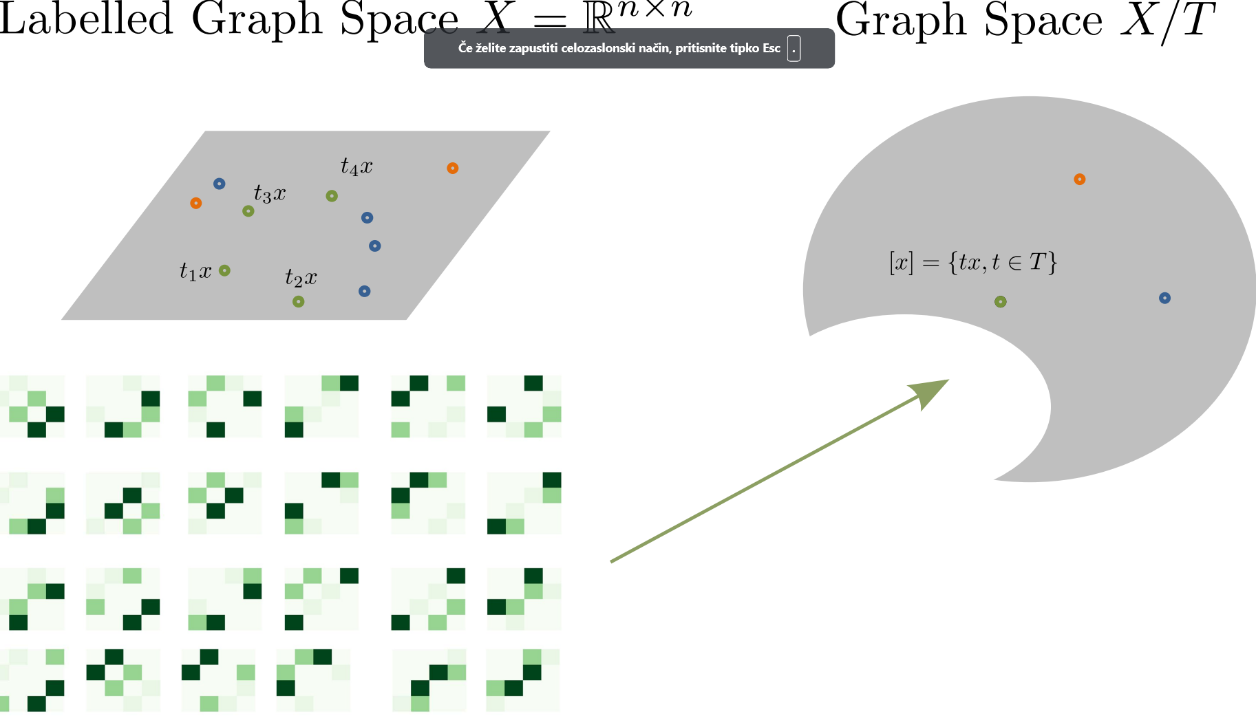
Figure 1: Conceptual visualization of Graph Space.
By equipping the total space with a metric \((X,d_X)\) we can define a quotient metric on \(X / T\) as: \[d_{X/T}([x_1],[x_2])=min_{t\in T}d_X (t^T x_1 t, x_2)\] Such metric corresponds in finding the optimal candidate in the equivalence class which minimize the distance in the total space. The minimization problem is known as the Graph Matching problem, which is a broadly studied problem in optimization (see Conte et al. (2004) for a review). As we select \(d_X\) to be the Frobenius norm, we use the FAQ Graph matching (Vogelstein et al. (2015)).
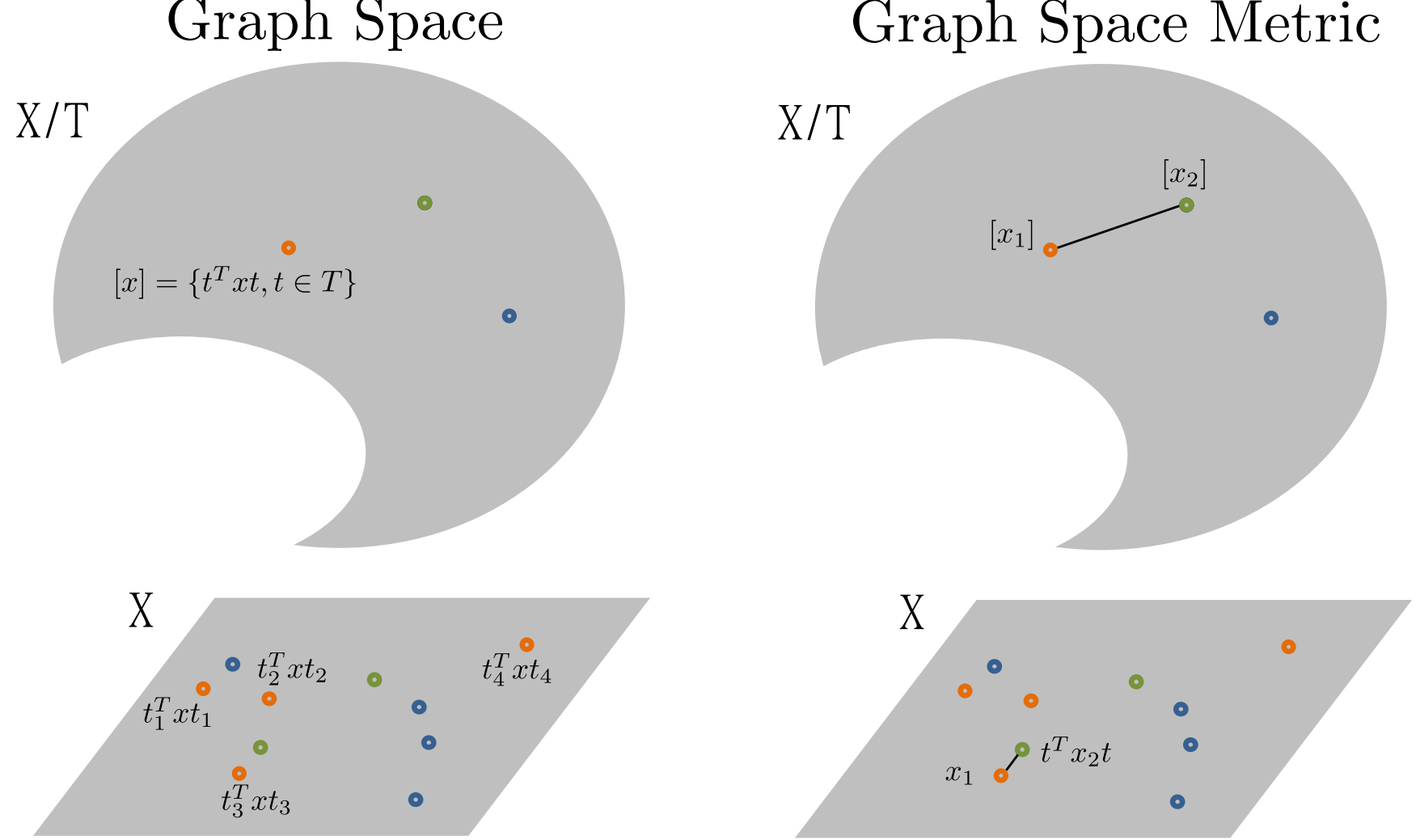
Figure 2: Conceptual visualization of the distance in the Graph Space.
Short Geometrical Characterization of Graph Space
The graph space is a metric space \((X / T,d_{X/T})\), but it is not a manifold: The equivalence classes are often not of the same dimensions (symmetries or blocks of zeros can cause the permutation to leave the graph unchanged), thus the action is not free and the space is not a quotient manifold (see Lee (2013) for details on quotient manifolds). However, the total space \(X=\mathbb{R}^{n\times n}\) is Euclidean. To overcome the complexity of the Graph Space and perform statistics on unlabelled graphs, we define an algorithm relying on the total space \(X\) for the computations.
Align All and Compute
The Align All and Compute Algorithm (AAC) allows to compute intrinsic statistics on Graph Space by computing the estimators on the total space. We illustrate it here for the estimation of the Fréchet Mean (Fréchet (1948)). Consider a set of \(\{[x_1],\dots,[x_k]\}\) graphs: \[[\bar{x}]=min_{[x]\in X / T }\sum_{i=1}^{n}d_{X /T}([\bar{x}],[x_i])\] Notice that the Fréchet Mean results into the arithmetic mean in the case of Euclidean data.
The AAC operates as follows:
AAC algorithm for the the Fréchet Mean
- Input: \(\{[x_1],\dots,[x_k]\} \subset X/T\); a threshold
\(\varepsilon > 0\)
- Initialization: Randomly select
\(\tilde{x}=\tilde{x_i}\in [x_i] \in \{ [x_1],\dots,[x_k]\}\)
- While \(s>\varepsilon\):
Obtain \(\tilde{x_i}\) optimally aligned wrt \(\tilde{x}\) for
\(i =\{ 1,\dots, k\}\)
Compute the Fréchet Mean \(\bar{x}\) in \(X\) of
\(\{\tilde{x_1},\tilde{x_2},\dots,\tilde{x_k}\} \in X\)
Compute \(s=d(\tilde{x},\bar{x})\)
Set \(\tilde{x}=\bar{x}\)
- Output: \([\bar{x}]\), an estimate of the Fréchet Mean of
\(\{[x_1], \ldots, [x_k]\} \in X/T\).
The Figure 3 represents the algorithm graphically:
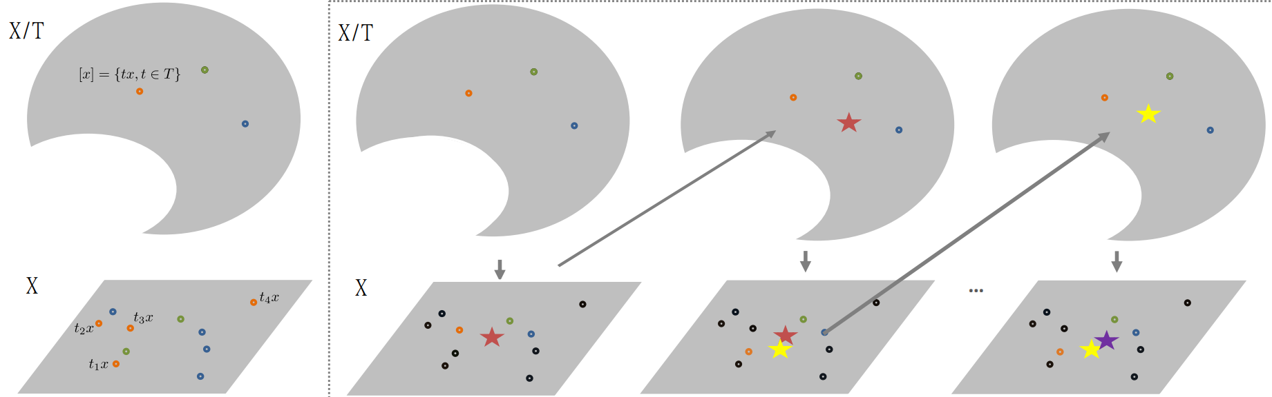
Figure 3: Conceptual visualization of the AAC algorithm. The star represents the current estimation of the Frechet Mean.
Generalized Geodesic Principal Components
Let’s move now to more complex estimators. To extend the Principal Component Analysis to Graph Space: (1) we firstly extend the concept of geodesic to Graph Space; (2) we define a way to align an equivalent class to a geodesic (i.e. optimal positioning).
Definition 1 (Generalized Geodesics):
Denote by \(\Gamma(X)\) the set of all straight lines (geodesics) in
\(X\). Following Huckemann, Hotz, and Munk (2010), a curve \(\delta\) is a generalized geodesic
on the Graph Space \(X/T\), if it is a projection of a straight line on
\(X\): \[\begin{equation}
\Gamma(X/T)=\{\delta=\pi \circ \gamma:\gamma\in\Gamma(X)\}.
\end{equation}\] Where \(\pi: X\rightarrow X/T\) is the canonical
quotient space projection.
Since Graph Space is not an inner product space, we define orthogonality as:
Definition 2: Two generalized geodesics \(\delta_1,\delta_2\in\Gamma(X/T)\) are orthogonal if they have representatives in \(\delta_1=\pi\circ\gamma_1,\delta_2=\pi\circ\gamma_2, \gamma_1,\gamma_2\in\Gamma(X)\) which are orthogonal \(<\gamma_1,\gamma_2>_X=0\).
In order to bridge computations in Graph Space \(X/T\) with computations in the total space \(X\), we introduce a concept of alignment in \(X\).
Definition 3 (Optimal position):
Given \(\tilde{x} \in X\) and \(t \in T\), the point \(t^T \tilde{x} t\)
is in if \[
d_X(t^T \tilde{x}t,x)= d_{X/T}([\tilde{x}],[x]).
\] That is, the equivalence class \([\tilde{x}] \in X/T\) contains (at
least) one point \(t^T \tilde{x} t \in [\tilde{x}]\) which has minimal
distance to \(x\), and this point is in optimal position to \(x\). Next,
consider \([x] \in X/T\), \(t \in T\) and \(\delta\) a generalized
geodesic in \(X/T\) with representative \(\gamma\in \Gamma(X)\). The
graph representative \(t^T x t\in X\) is in optimal position to
\(\gamma\in\Gamma(X)\) if \[d_X(t^T x t ,\gamma)=d_{X/T}([x],\delta).\]
Having concepts of generalized geodesic, optimal position and orthogonality, we now define a set of geodesic principal components:
Definition 4: Consider the canonical projection of the Graph Space \(\pi \colon X \rightarrow X/T\) of \(X\) and consider a set \(\{[x_1],\dots, [x_k]\} \subset X/T\) of graphs, \([x]\in X/T\), and \(\delta \in \Gamma(X/T)\). The Generalized Geodesic Principal Components (GGPCs) for the set \(\{[x_1],\dots, [x_k]\}\) are defined as:
The first generalized geodesic principal component \(\delta_1 \in \Gamma(X/T)\) is the generalized geodesic minimizing the sum of squared residuals: \[\begin{equation}\label{eq:wrtdelta} \delta_1 = \underset{\delta \in \Gamma(X/T)}{\operatorname{argmin}} \sum_{i=1}^{k}{(d_{X/T}^2([x_i],\delta))} \end{equation}\]
The second generalized geodesic principal component \(\delta_2 \in \Gamma(X/T)\) minimizes (2) over all \(\delta \in \Gamma(X/T)\), having at least one point in common with \(\delta_1\) and being orthogonal to \(\delta_1\) at all points in common with \(\delta_1\).
The point \(\mu\in X/T\) is called Principal Component Mean if it minimizes \[\begin{equation}\label{eq:wrtpoint} \sum_{i=1}^{k}{(d_{X/T}^2([x_i],[\mu])^2)} \end{equation}\] where \([\mu]\) only runs over points \(\tilde{x}\) in common with \(\delta_1\) and \(\delta_2\).
The \(j^{th}\) generalized geodesic principal component is a \(\delta_j \in \Gamma(X/T)\) if it minimizes (2) over all generalized geodesics that meet orthogonally \(\delta_1,\dots, \delta_{j-1}\) and cross \(\mu\).
Conceptualized in Figure 4, the actual estimation of the GPCA in Graph Space is done via AAC: (1) Randomly pick some candidates in the equivalence classes; (2) estimate the standard PCA in \(X\); (3) Select new optimally aligned candidates wrt the current PCA estimation.
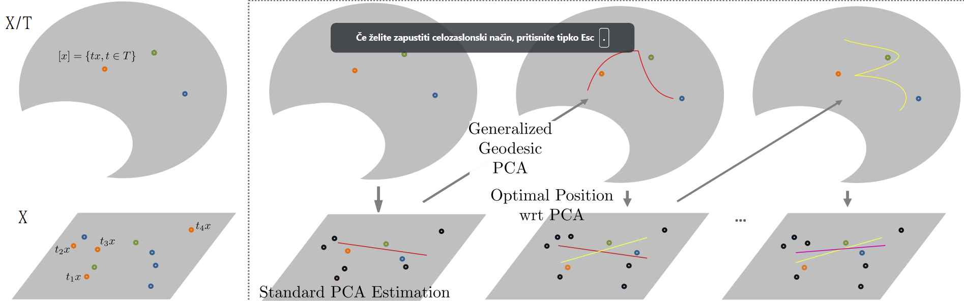
Figure 4: Conceptual visualization of the AAC for the estimation of the first generalized geodesic principal component.
The AAC converge in finite time and to a local minima as proven in Theorem 2 and 3 (Calissano, Feragen, and Vantini (2023)). All the algorithms and the framework is implemeted in the geomstats python package.
An Example
As an intuitive visual example with real data and associated vectors attributes, we subsample \(20\) cases of the letter A from the well known hand written letters dataset (Kersting et al. (2016), Riesen and Bunke (2008)). As shown in the left panel of Figure 5, every network has node attributes consisting of the node’s \(x\)- and \(y\)-coordinates, and binary \((0/1\)) edge attributes indicating whether nodes are connected by lines.
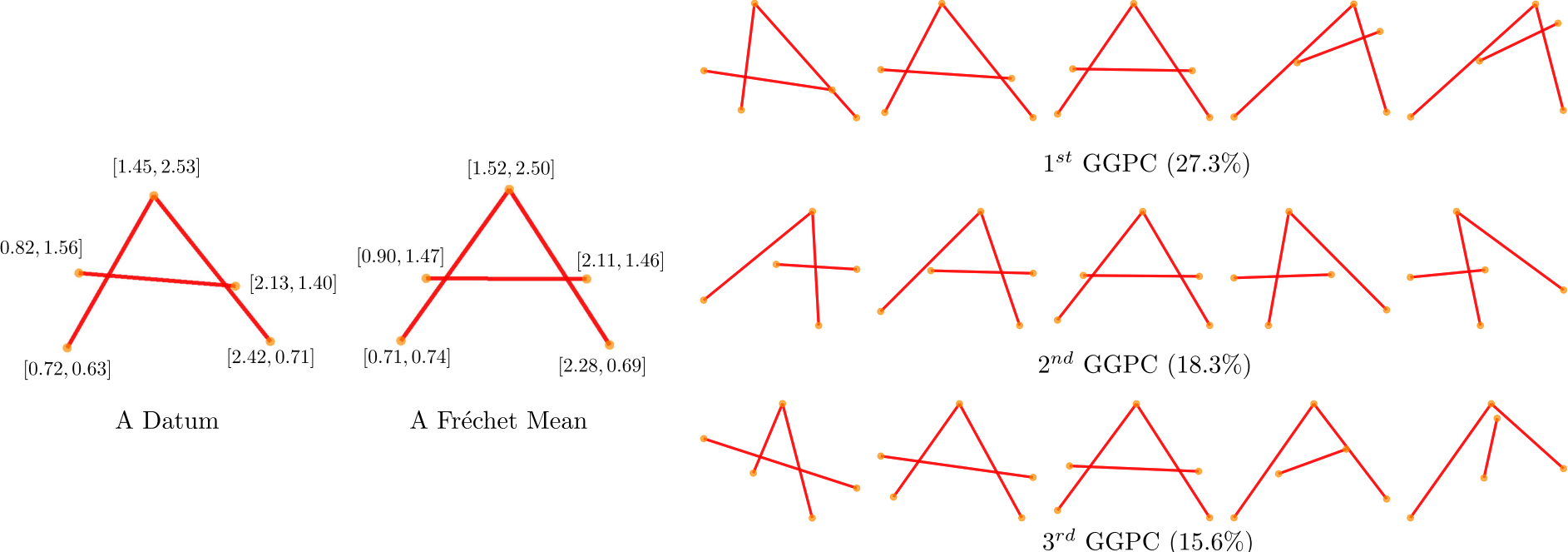
Figure 5: Left: A datum extracted from the \(A\) dataset. Every unlabelled node has a bi-dimensional real valued attribute, while every edge has a \({0,1}\) attribute. The Fréchet mean. Right: Visualization of the GGPCs. \({0.1,0.25,0.5,0.75,0.9}\) quantile of the projected scores are shown for the first three GGPCs.
Conclusion
Graph Space is an intuitive embedding for sets of graphs with unlabelled sets of nodes. Even if its geometry is far from trivial, we can easily estimate intrinsic statistics by using the Align All and Compute algorithm. In Calissano, Feragen, and Vantini (2023) we detailed the geometry of Graph Space, we define the AAC algorithm and the Generalized Geodesic Principal Components for a set of graphs. Regression with unlabelled network outputs is also available in Calissano, Feragen, and Vantini (2022). All the framework is available as part of the geomstats python package (Miolane et al. (2020)).