Overview
In this post we present a new estimation procedure for functional linear regression useful when the regression surface – or curve – is supposed to be exactly zero within specific regions of its domain. Our approach involves regularization techniques, merging a B-spline representation of the unknown coefficient function with a peculiar overlap group lasso penalty. The methodology is illustrated on the well-known Swedish mortality dataset and can be employed by \({\tt R}\) users through the package \({\tt fdaSP}\).
Introduction
We consider the framework on which a functional response \(y_i(s)\) with \(s \in \mathcal{S}\) is observed together with a functional covariate \(x_i(t)\) with \(t \in \mathcal{T}\) for \(i=1, \dots, n\). The simplest modeling strategy for function-on-function regression is the concurrent model, which assumes that \(\mathcal{T} = \mathcal{S}\) and the covariate \(x(\cdot)\) influences \(y(s)\) only through its values \(x(s)\) at the domain point \(s \in \mathcal{S}\). The relation when both variables are centered is given by
\[ y_i(s) = x_i(s)\psi(s) + e_i(s)\]
where \(\psi(s)\) is the regression function and \(e_i(s)\) is a functional zero-mean random error. The more general approach, named nonconcurrent functional linear model, allows \(y_i(s)\) to entirely depend on the functional regressor in the following way
\[ y_i(s) = \int_{\mathcal{T}} x_i(t) \psi(t, s) dt + e_i(s) . \] The model allows \(\mathcal{T} \neq \mathcal{S}\) and the bivariate function \(\psi(t, s)\) represents the impact of \(x(\cdot)\) evaluated at \(t \in \mathcal{T}\) on \(y_i(s)\) and usually is a “dense” function. Our goal is to introduce a nonconcurrent functional linear model that allows for local sparsity patterns. Specifically, we want that \(\psi(t, s) = 0\) for \((t, s) \in \mathcal{D}_0\) with \(\mathcal{D}_0\) being a suitable subset of the domain \(\mathcal{D}\) of \(\psi(\cdot)\), with \(\mathcal{D} = \mathcal{S} \times \mathcal{T}\), thus, inducing locally sparse Hilbert-Schmidt operators. Note that the set \(\mathcal{D}_0\) is unknown and need to be estimated from data.
Locally sparse functional model
B-splines and sparsity
In order to represent functional objects using basis expansion, we select a basis \(\{\theta_l(s), l = 1, \dots , L\}\) of dimension \(L\) in the space of square integrable functions on \(\mathcal{S}\) and a basis \(\{\varphi_m(t), m = 1, \dots ,M\}\) of dimension \(M\) in the space of square integrable functions on \(\mathcal{T}\). Exploiting a tensor product expansion of these two, we represent the regression coefficient \(\psi\) as
\[\begin{eqnarray} \psi(t,s) & = \sum_{m=1}^M \sum_{l=1}^L \psi_{ml} \varphi_m(t) \theta_l(s) = & (\varphi_1(t), \dots, \varphi_M(t)) \left( \begin{matrix} \psi_{1,1} & \cdots & \psi_{1,L} \\ \vdots & \ddots& \vdots \\ \psi_{M,1} & \cdots & \psi_{M,L} \end{matrix}\right) \left( \begin{matrix} \theta_{1}(s)\\ \vdots \\ \theta_{L}(s) \end{matrix}\right) = \boldsymbol{\varphi}(t)^T \boldsymbol{\Psi} \boldsymbol{\theta}(s), \label{eq:tensorproduct} \end{eqnarray}\]
where \(\psi_{ml} \in \mathbb{R}\) for \(l=1, \dots, L\) and \(m=1, \dots, M\). A key point is to assume that elements in this representation are B-splines (De Boor 1978) of order \(d\) with \(L − d\) and \(M − d\) interior knots, respectively. Suitable zero patterns in the B-spline basis coefficients of \(\boldsymbol{\Psi}\) induce sparsity in \(\psi(t, s)\). Let \(\tau_1 < \dots < \tau_m < \dots < \tau_{M−d+2}\) and \(\sigma_1 < \dots < \sigma_l < \dots < \sigma_{L−d+2}\) denote the knots defining the tensor product splines, with \(\tau_1, \tau_{M−d+2}\) and \(\sigma_1, \sigma_{L−d+2}\) being the boundaries of the two domains, and let \(\mathcal{D}_{ml} \in \mathcal{D}\) be the rectangular subset of \(\mathcal{D}\) defined as \(\mathcal{D}_{ml} = (\tau_m, \tau_{m+1}) \times (\sigma_l, \sigma_{l+1})\) for \(m = 1, \dots ,M − d + 1\) and \(l = 1, \dots , L − d + 1\). To obtain \(\psi(t, s) = 0\) for each \((t, s) \in \mathcal{D}_{ml}\), it is sufficient that all the coefficients \(\psi_{m'l'}\) with \(m' = m, \dots ,m + d − 1\) and \(l' = l, \dots , l+d−1\) are jointly zero. The following figure further clarifies this concept.
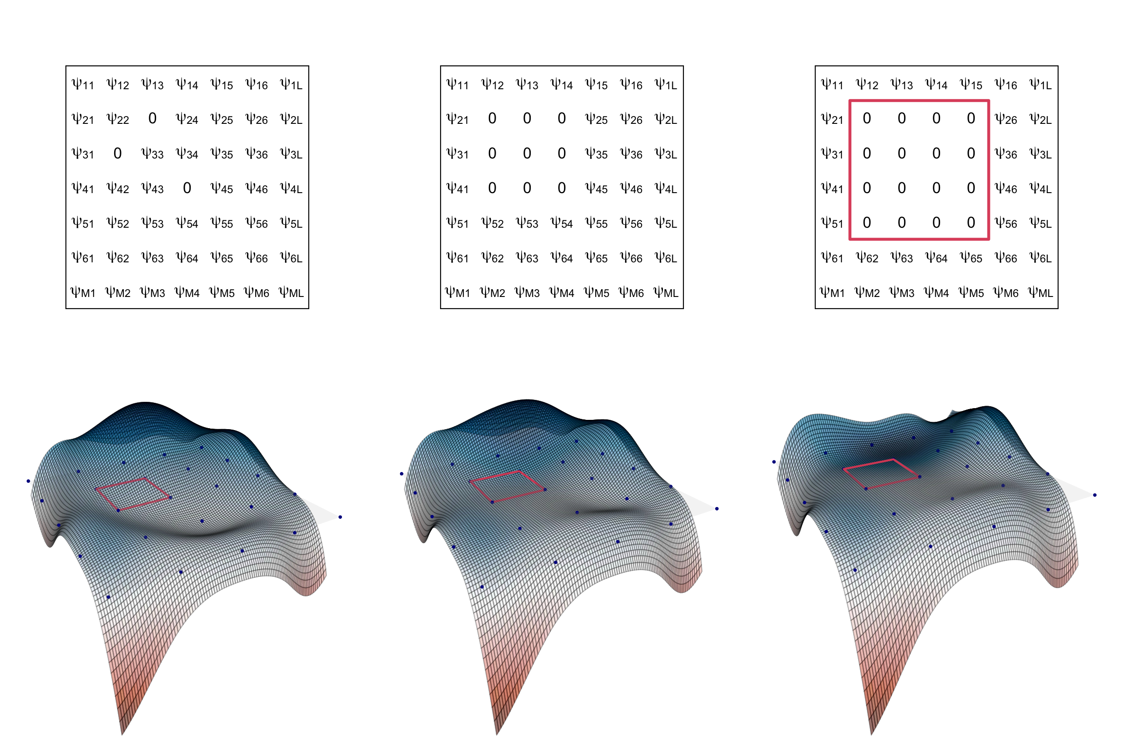
Bivariate example with tensor product cubic B-splines (d=4). The top row shows different coefficient matrix patterns, while the bottom row shows the corresponding spline, where dots represent knots and the set D is highlighted in red. The first 2 columns show a coefficient matrix with isolated zeros and a (d-1) x (d-1) block of zeros, respectively. None of the two is able to produce a sparse function. In the last column, conversely, an entire d x d block of coefficients is null and the resulting function is indeed sparse.
The previous figure suggests that, in general, \(\psi(t, s)\) equals zero in the region identified by two pairs of consecutive knots if the related \(d\) × \(d\) block of coefficients of \(\boldsymbol{\Psi}\) is entirely set to zero. Therefore, \(\boldsymbol{\Psi}\) should be suitably partitioned in several blocks of dimensions \(d\) × \(d\) on which a joint sparsity penalty is induced.
Note that in the simpler situation where a functional covariate \(x_i(t)\) and a scalar response \(y_i\) are observed we have the following simplifications. The functional linear model is
\[ y_i = \int x_i(t) \psi(t) dt + e_i, \] the regression function is expanded as \(\psi(t) = \sum_{m=1}^M \psi_m \varphi_m(t)\) and the set \(\mathcal{D}_m = (\tau_m, \tau_{m+1})\) is an interval of the real line. To obtain \(\psi(t) = 0\) for each \(t \in \mathcal{D}_{m}\), it is sufficient that all the coefficients \(\psi_{m'}\) with \(m' = m, \dots ,m + d − 1\) are jointly zero and \(\psi(t)\) equals zero in the interval identified by two pairs of consecutive knots if the related \(d-\)dimensional subvector of coefficients is entirely set to zero. This behaviour is illustrated in the next figure.
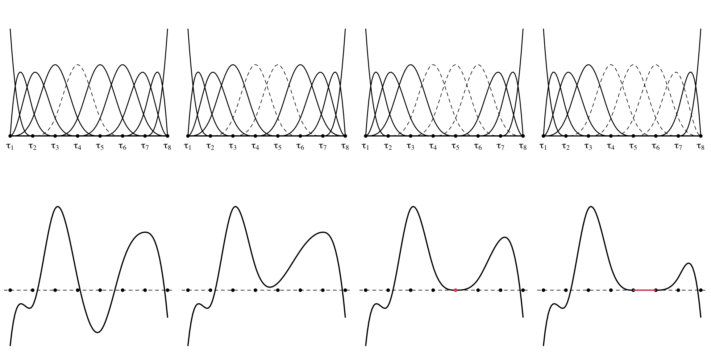
Univariate cubic B-spline basis and resulting spline functions. Dashed curves correspond to bases with a zero-valued coefficient. Only in the case when d=4 consecutive coefficients are zero the resulting spline function is null on a set of positive Lebesgue measure (in red).
Overlap group Lasso
Having in mind the above mentioned B-splines sparsity properties, in order to estimate a locally-sparse regression surface, we minimize the following objective function
\[ \frac{1}{2} \sum_{i=1}^n \int \bigg( y_i(s) - \int x_i(t)\psi(t,s) dt \bigg)^2 ds + \lambda \Omega(\boldsymbol{\Psi}), \]
but, instead of specifying the functional form for the penalty \(\Omega(\cdot)\) as the widely-employed Lasso (Tibshirani, 1996) or group-Lasso (Yuan and Lin, 2006) that would not work properly (see paper for details), we propose to use something truly tailored for the problem. First, instead of a disjoint partition, we define an overlapping sequence of blocks of size \(d\) × \(d\). Specifically, we introduce the block index \(b = 1, \dots , B\) with the total number of blocks denoted by \(B = (M − d + 1) \times (L − d + 1)\). Notably, there is a block for each set \(\mathcal{D}_{ml}\). This overlapping group structure allows \(\mathcal{D}_0\) to be the union of any set \(\mathcal{D}_{ml}\) by moving a block of minimum size. An example of overlapping covering when \(d=4\) (cubic splines) is shown in the following figure.
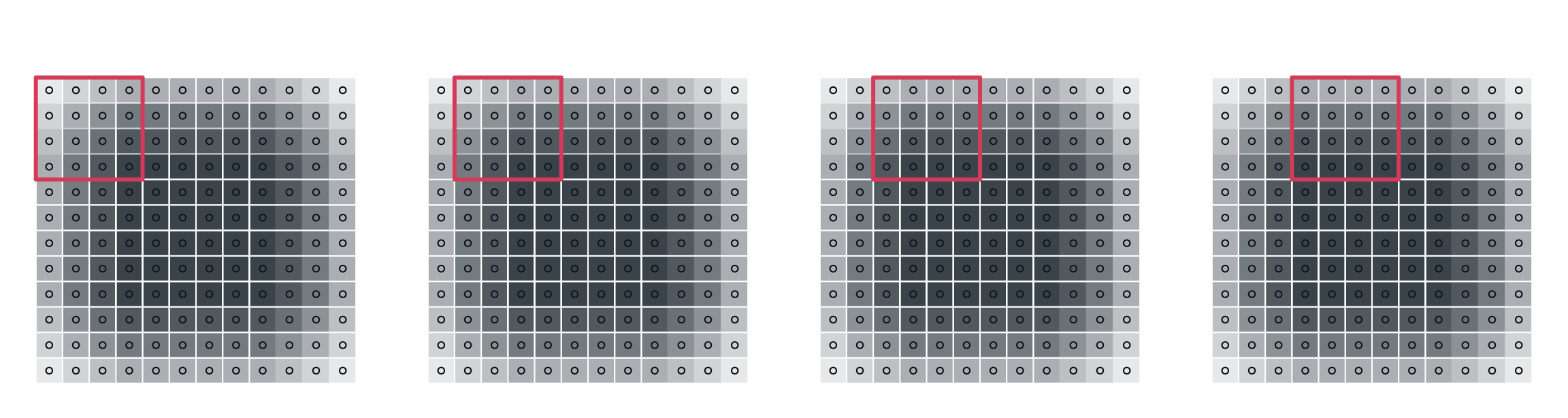
Overlapping covering of the coefficient matrix (L = M = 12) with the first 4 blocks of size d × d, d = 4. Colors according to the balancing vector.
This construction suggests specifying a penalty \(\Omega\) for overlapping groups of coefficients, which has attracted significant interest in the last decade, see Jacob, Obozinski and Vert (2009), Jenatton, Audibert and Bach (2011) and Lim and Hastie (2015). Being interested in the sparsity structure of the matrix of coefficients \(\boldsymbol{\Psi}\) rather than its support we particularize the previous problem as
\[ \frac{1}{2} \sum_{i=1}^n \int \left( y_i(s) - \int x_i(t) \psi(t,s) dt \right)^2 ds + \lambda \sum_{b=1}^{B+1} || c_{b} \odot \boldsymbol{\psi} ||_2, \]
where \(\lambda > 0\) is a fixed penalization term, and \(\Omega\) specifies in the sum of \(B + 1\) Euclidean norms \(\lVert c_b \odot \boldsymbol{\psi} \rVert_2\), where \(\boldsymbol{\psi} = \text{vec}(\boldsymbol{\Psi})\), and \(\odot\) represents the Hadamard product. The index \(b\) denotes the block of coefficients in \(\boldsymbol{\Psi}\), with the first \(B\) blocks being consistent with the aforementioned construction and the last block containing all coefficients in \(\boldsymbol{\Psi}\). Vectors of size \(ML\), denoted by \(c_b\), are needed to extract the correct subset of entries of \(\boldsymbol{\Psi}\) and contain also known constants that equally balance the penalization of the coefficients. This balancing is needed because the parameters close to the boundaries appear in fewer groups than the central ones. Note that this penalty constitutes a special case of the norm defined by Jenatton, Audibert, and Bach (2011).
In the case of a scalar response, the objective function becomes
\[ \frac{1}{2} \sum_{i=1}^n \left( y_i - \int x_i(t) \psi(t) dt \right)^2 + \lambda \sum_{b=1}^{B+1} || c_{b} \odot \boldsymbol{\psi} ||_2 \]
where \(\boldsymbol{\psi}\) and \(c_b\) are vectors of dimension \(M\) and each of the first \(B\) blocks contains \(d\) consecutive coefficients, as in the following example.
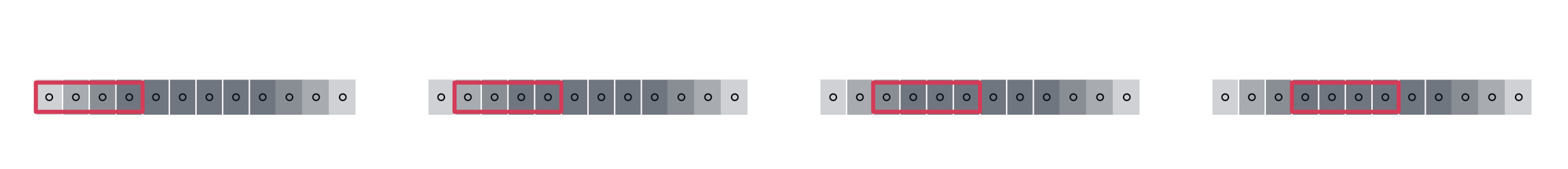
Overlapping covering of the coefficient vector (M = 12) when the response is scalar with the first 4 blocks of size d = 4. Colors according to the balancing vector.
Computational Considerations
To develop an efficient computational strategy, we introduce the empirical counterparts of the quantities described in the previous section assuming to observe a sample of response curves \(y_i\) with \(i=1, \dots,n\) on a common grid of \(G\) points, i.e. \(y_i = (y_i(s_1), \dots, y_i(s_G))^T\). Let also \(x_i\) be the related functional covariate observed on a possibly different but— common across \(i\)—grid of points, that for simplicity and without loss of generality, we assume of length \(G\). Let \(\mathbf{X}\) be the \(n \times G\) matrix with \(x_i\) in the rows. Let \(\boldsymbol{\Phi}\) and \(\boldsymbol{\Theta}\) be the \(M \times G\) and \(L \times G\) matrices defined as \[ \boldsymbol{\Phi} = \begin{pmatrix} \varphi_1(t_1) & \cdots & \varphi_1(t_G) \\ \vdots&&\vdots \\ \varphi_m(t_1) & \cdots & \varphi_m(t_G) \\ \vdots&&\vdots \\ \varphi_M(t_1) & \cdots & \varphi_M(t_G) \\ \end{pmatrix}, \quad \quad \boldsymbol{\Theta} = \begin{pmatrix} \theta_1(s_1) & \dots & \theta_1(s_G) \\ \vdots&&\vdots \\ \theta_l(s_1) & \cdots & \theta_l(s_G) \\ \vdots&&\vdots \\ \theta_L(s_1) & \cdots & \theta_L(s_G) \\ \end{pmatrix}, \] and let \(\mathbf{Y}\) and \({\bf E}\) be the \(n\times G\) matrices obtained as \(\mathbf{Y} = (y_1, \dots, y_n)^T\) and \(\mathbf{E} = (e_1, \dots, e_n)^T\) , with \(e_i = (e_i(s_1), \dots, e_i(s_G))^T\). The function-on-function linear regression model can be equivalently written in matrix form as \[ \mathbf{Y} = \mathbf{X} \boldsymbol{\Phi}^T \boldsymbol{\Psi} \boldsymbol{\Theta} + {\bf E}. \]
Applying the vectorization operator on each side of the equality above, we obtain the new optimization problem
\[ \frac{1}{2}\Vert \mathbf{y} - \mathbf{Z} \boldsymbol{\psi}\Vert_2^2 + \lambda \sum_{b=1}^{B+1} \Vert \mathbf{D}_{b}\boldsymbol{\psi} \Vert_2, \]
where \(\mathbf{y}=\text{vec}(\mathbf{Y})\), \(\boldsymbol{\psi}=\text{vec}(\boldsymbol{\Psi})\) is the vector of coefficients of dimension \(LM\), \(\mathbf{Z} = \boldsymbol{\Theta}^T \otimes \mathbf{X} \boldsymbol{\Phi}^T\) and \(\mathbf{D}_b=\mathrm{diag}(c_b)\) is a diagonal matrix whose elements correspond to the elements of the vector \(c_b\). The minimization of the quantity above is challenging because of the non-separability of the overlap group Lasso penalty. We propose a Majorization-Minimization (MM) algorithm (Lange, 2016) to obtain the solution, although other choices are viable e.g., the Alternating Direction Method of Multipliers (ADMM), see Boyd et al. (2011). The MM procedure works in two steps: in the first step a majorizing function \(\mathcal{Q}(\boldsymbol{\psi}\vert\widehat{\boldsymbol{\psi}}^{k})\) based on the actual estimate is determined and in the second step this function is minimized. Alternating between the two guarantees the convergence to a solution of the original problem. The curious reader can find the expression of \(\mathcal{Q}(\boldsymbol{\psi}\vert\widehat{\boldsymbol{\psi}}^{k})\) in the original paper, here we just point out that the function is quadratic and admits an explicit solution in the form of generalized ridge regression. A further speed-up, when the dimension of the problem is high, is made exploiting the Sherman-Morrison-Woodbury matrix identity, also known as the matrix inversion lemma.
When the response is scalar, we have the following modifications. The design matrix is \(\mathbf{Z} = \mathbf{X} \boldsymbol{\Phi}^T\), \(\mathbf{y}\) and \(\boldsymbol{\psi}\) are vectors of dimension respectively \(n\) and \(M\) and the diagonal matrix \(\mathbf{D}_{b}\) is of dimension \(M \times M\). The optimization problem is still valid and the same class of algorithms can be employed to obtain the solution.
Swedish mortality revisited
We apply the proposed locally sparse estimator to the Swedish mortality dataset, where the aim is to predict the log-hazard function on a given year from the same quantity on the previous year. We implement the model with \(d = 4, M = L = 20\) basis functions on each dimension and select the optimal value of \(\lambda\) by means of cross-validation. A perspective plot of the estimated surface is depicted in the last figure of the post. The estimate shows a marked positive diagonal confirming the positive influence on the log-hazard rate at age \(s\) of the previous year’s curve evaluated on a neighborhood of \(s\). At the same time, the flat zero regions outside the diagonal suggest that there is no influence of the curves evaluated at distant ages. Our estimate is more regular than previous approaches and its qualitative interpretation sharper and easier. Refer, for example, to Figure 10.11 of Ramsay, Hooker, and Graves (2009).
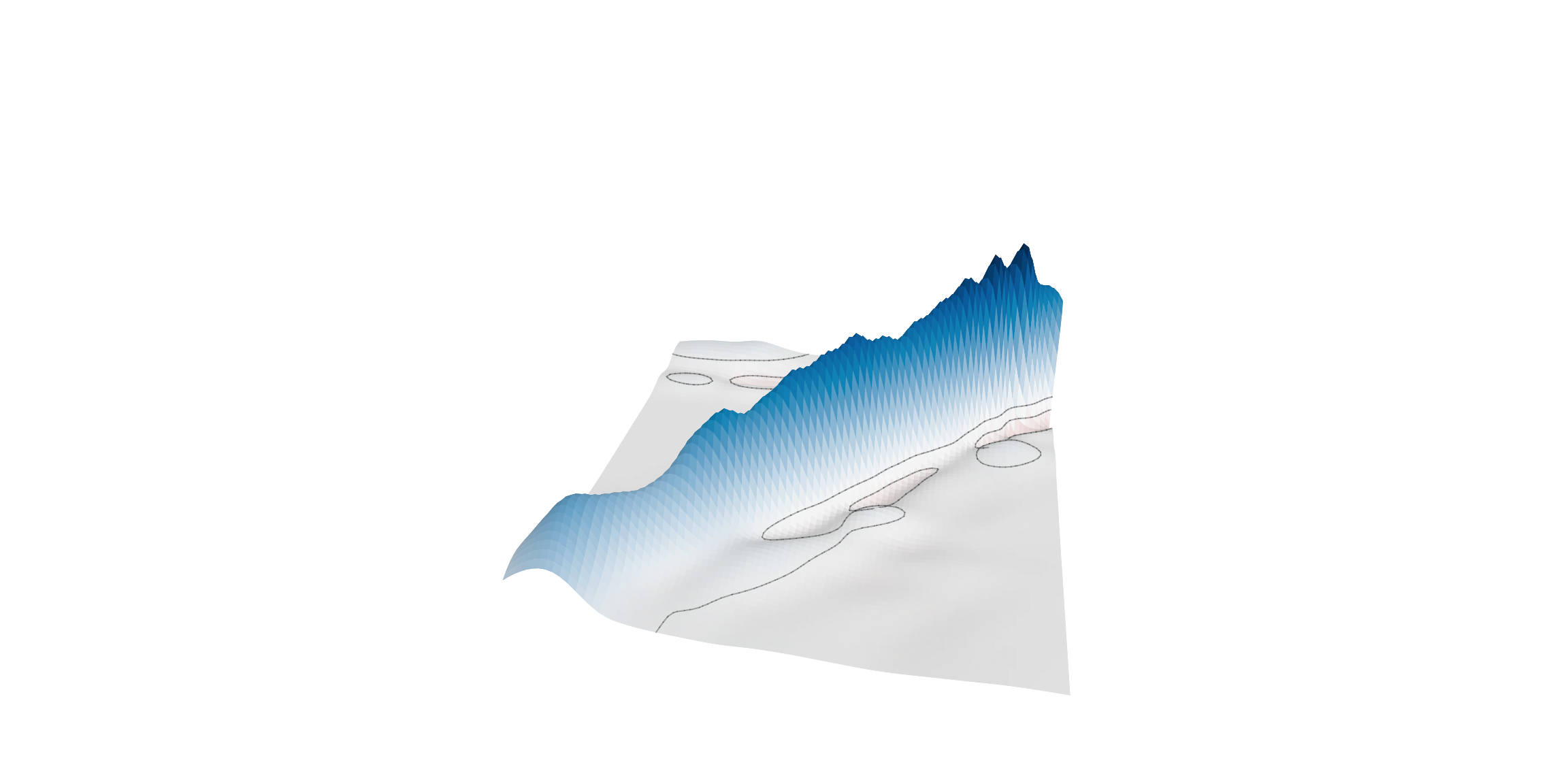
Estimated regression surface for the Swedish mortality dataset.
This result witnesses the practical relevance of adopting the proposed approach. Indeed, the resulting estimate, while being reminiscent of a concurrent model—inheriting its ease of interpretation—gives further insights and improves the fit, representing the desired intermediate solution between the concurrent and nonconcurrent models.
\({\tt R}\) package
The method is implemented in \({\tt R}\) through the package \({\tt fdaSP}\), available on CRAN. The function \({\tt f2fSP}\) can be used for a functional response regression model while \({\tt f2sSP}\) for a scalar response one. The two counterparts \(\texttt{f2fSP_cv}\) and \(\texttt{f2sSP_cv}\) are useful to select the tuning parameter by means of cross-validation.
This post is based on
Bernardi, M., Canale, A. and Stefanucci, M. (2022). Locally Sparse Function-on-Function Regression, Journal of Computational and Graphical Statistics, 32:3, 985-999, DOI: 10.1080/10618600.2022.2130926
References
Tibshirani, R. (1996), “Regression Shrinkage and Selection via the
Lasso,” Journal of the Royal Statistical Society, Series B, 58,
267–288.
Yuan, M., and Lin, Y. (2006), “Model Selection and Estimation in
Regression with Grouped Variables,” Journal of the Royal Statistical
Society, Series B, 68, 49–67.
Jacob, L., Obozinski, G., and Vert, J.-P. (2009), “Group Lasso with
Overlap and Graph Lasso,” in Proceedings of the 26th Annual
International Conference on Machine Learning, pp. 433–440.
Jenatton, R., Audibert, J.-Y., and Bach, F. (2011), “Structured Variable
Selection with Sparsity-Inducing Norms,” Journal of Machine Learning
Research, 12, 2777–2824.
Lim, M., and Hastie, T. (2015), “Learning Interactions via Hierarchical
Group-Lasso Regularization,” Journal of Computational and Graphical
Statistics, 24, 627–654.
Lange, K. (2016), “MM optimization algorithms.” Society for Industrial
and Applied Mathematics, Philadelphia, PA.
Boyd, S., Parikh, N., Chu, E., Peleato, B. and Eckstein, J. (2011),
“Distributed optimization and statistical learning via the alternating
direction method of multipliers,” Foundations and Trends® in Machine
Learning, 3, 1–122.
Ramsay, J. O., Hooker, G., and Graves, S. (2009), Functional Data
Analysis with R and Matlab, NewYork: Springer.