In the following we show how it is possible to obtain parallelizable, unbiased and computationally cheap estimates of Crossed random effects models with a linear cost in the number of datapoints (and paramaters) exploiting couplings.
Crossed random effects models (CREM)
CREM model a continuous response variables \(Y\) as depending on the sum of unknown effects of \(K\) categorical predictors. Think of the \(Y_n\) as the ratings given to university courses, along with some factors potentially impacting such a score, e.g. student identity, code of the course, department teaching it, professors ecc. Aim of the model is investigating the effect of each of those factors on the overall score. In their simplest version (i.e. linear, intercept-only case), the model takes the form:
\[\begin{equation} \label{eq:crem} \mathcal{L}(y_n) = f \left(\mu +\sum_{k=1}^K a_{i_{k[n]}}^{(k)},\tau_0^{-1}\right) \text{ for } n=1,...,N, \end{equation}\] where \(f\) indicates the density of some distribution whose mean is the sum of \(\mu\), a global mean, and \(a^{(k)}_{i_{k[n]}}\), i.e. the unknown effects of the student identity, the department teaching it ecc.
We are interested in studying how the cost of estimating the unknown effects scales as the number of observations \(N\) and of parameters \(p\) grows to \(\infty\). Our goal is an algorithm whose complexity scales linearly in \(N\) and \(p\), and we call such algorithms “scalable”. Both in the Frequentist and in the Bayesian literature, these models are difficult to estimate: works of Gao and Owen (2016a) and Gao and Owen (2016b) showed how the “vanilla” implementation of GLS and of Gibbs samplers have a computational cost that grows at best as \(O(N^\frac{3}{2})\). Recent works by Papaspiliopoulos, Roberts, and Zanella (2019) and Ghosh, Hastie, and Owen (2022) proposed, respectively, a collapsed Gibbs sampler and a “backfitting” iterative algorithm that exhibit computational costs linear in the number of observations; in particular the MCMC induced by the collapsed scheme is proved to have a mixing time that is \(O(1)\) under certain asymptotic regimes.
It is possible to further improve the MCMC estimates exploiting couplings: as showed in Jacob, O’Leary, and Atchadé (2020) and Glynn and Rhee (2014), coupling two MCMC chains allows to derive unbiased estimators of posterior quantities, provided that the two coupled chains are exactly equal after a finite number of iterations. Furthermore, the same construction provides theoretical foundations for the early stopping of the chains (once met) and allows for the parallelization of independent experiments.
The extra computational cost one has to pay is represented by the product between the cost of each iteration and the expected number of iterations needed for coalescence. As for the former, it is possible to devise many coupling algorithms for which the cost of each iteration is easily computable and linear in the number of observations. As for the expected meeting time, for chains arising from a Gibbs sampling scheme targeting Gaussian distributions, it is possible to show that is directly related to the mixing time of the single Markov chain, and indeed it differs from the latter only by a logarithmic factor up to some constants (see the Sections below for more details). Hence chains that mix fast also meet in a small number of iteration and therefore provide unbiased estimates with low computational cost.
Couplings for estimation
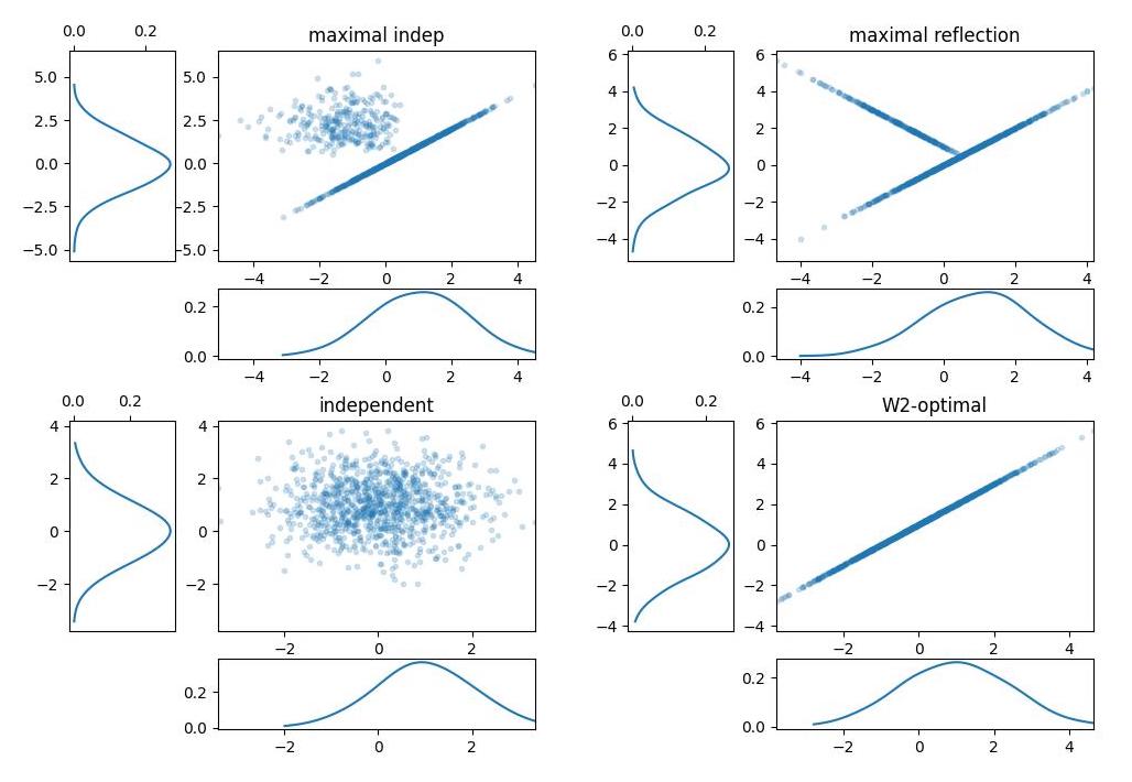
Theoretically speaking, given \(X,Y\) random variables distributed according to \(P,Q\) respectively, a coupling of the two is random variables \((X, Y)\) on the joint space such that the marginal distribution of \(X\) is \(P\) and the marginal distribution of Y is \(Q\). Clearly, given two marginal distributions, there are infinitely many joint distributions with those as marginals. Below some of the possible couplings of a \(N(1,1)\) (on the x-axis) and \(N(0,1)\) on the y-axis. Starting clockwise from top left: maximal independent (i.e. a coupling maximizing the probability of equal draws), maximal reflection, independent (bivariate independent normal) and \(W2\)-optimal (maximally correlated draws).
Couplings of Gaussian distributions
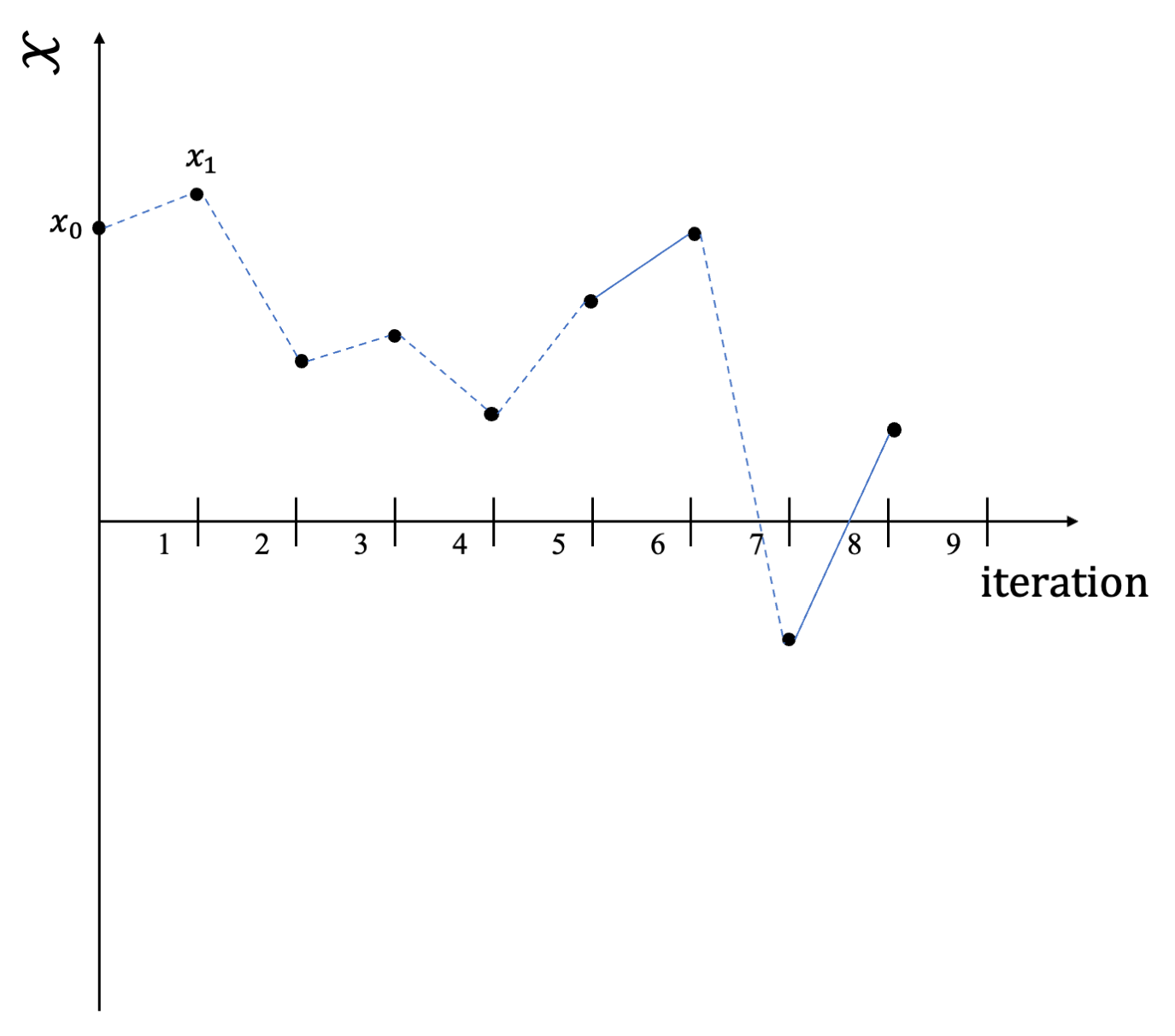
Couplings might be used for obtaining unbiased estimators in MCMC inference, as shown in Jacob, O’Leary, and Atchadé (2020). Given a target probability distribution \(\pi\) and an integrable function \(h\), we are interested in estimating: \[\mathbb{E}_{\pi}[h(\boldsymbol{\Theta})] = \int h(\boldsymbol{\theta}) \pi(d\boldsymbol{\theta}).\] Usually, one would sample a chain according to some Markov kernel \(P\), designed to leave the chain \(\pi\) invariant, i.e. a Gibbs kernel or random walk Metropolis (Hastings 1970). Below the sample path of such a chain.
Sample path of a single MC
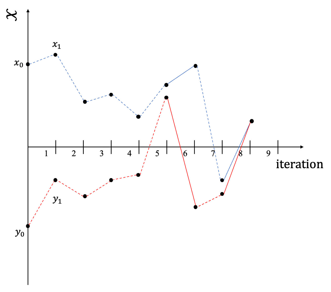
Instead of waiting until convergence, one could run two coupled Markov chains \((\boldsymbol{\Theta}^1_t)_{t\ge -1}\) and \((\boldsymbol{\Theta}^2_t)_{t \ge0}\), which marginally starts from some base distribution \(\pi_0\) and evolves according to the same kernel \(P\), but some correlation is induced in order to let the chains meet after an almost surely finite number of iterations. Basically at iteration \(t\) instead of sampling from \(X_{t+1} \sim P(X_t, \cdot)\) and \(Y_{t+1} \sim P(Y_t, \cdot)\) independently, we sample from a coupling of the two distributions.
Sample path of coupled MCs
Then, for any fixed \(m \ge k\), we can run coupled chains for \(\max(m, T)\) iterations and \(H_{k:m}\) is an unbiased estimator: \[\begin{align*} H_{k:m} & = \frac{1}{m-k+1} \sum_{l=k}^m h(\boldsymbol{\Theta}^1_l) + \sum_{l=k+1}^{\tau} \min \left(1, \frac{l-k}{m-k+1}\right) \left(h(\boldsymbol{\Theta}^1_l)-h(\boldsymbol{\Theta}^2_{l})\right) \\ &= MCMC_{k:m} + BC_{k:m}. \end{align*}\] The form of the estimator includes two terms: the first term corresponds to a standard MCMC average with \(m-k+1\) total iterations and \(k-1\) burn-in steps, and the other term is a “bias correction”, the part that corrects the bias present in the MCMC average.
For more details give a look up at https://sites.google.com/site/pierrejacob/cmclectures.
In order two yield small meeting times, we implement a “two-step” coupling strategy: whenever the chains are “far away” (in some notion that will be clarified later) use a coupling whose aim is to bring the realizations closer to each other; whenever “close enough”, choose a coupling maximizing the meeting probabilities. The heuristic for this construction is that whenever a maximal coupling fails, components are sampled far away in the space, thus reducing the coalescence probability for the next steps.
Bound on coupling time
Consider \((\boldsymbol{\theta}_t)_{t\ge 1}=(\boldsymbol{\theta}^1_t, \boldsymbol{\theta}^2_t)_{t\ge 0}\), two \(\pi\)-reversible Markov chains arising from a Gibbs sampler targeting \(\pi=N(\boldsymbol{\mu},\Sigma)\). If a “two-step” strategy is implemented, with maximal reflection and \(W2\) optimal couplings, then for every \(\delta >0\), the meeting time \(T\) is bounded by \[\begin{equation} \mathbb{E}[T| \boldsymbol{\theta}_0] \le 5 + 3 \max \left(n^*_\delta, T_{rel} \left[\frac{\ln(T_{rel})}{2} + C_0 + C_\varepsilon \right] (1+\delta) \right), \end{equation}\]on} where \(C_0\) denotes a constant solely depending on \(\boldsymbol{\theta}^1_0, \boldsymbol{\theta}^2_0\) and the posterior variance \(\Sigma\), \(C_\varepsilon\) depends on the fixed parameters \(\varepsilon\), and \(n^*_\delta = inf_{n_0} \{ n_0 \ge 1: \forall n \ge n_0 \; 1-\| B^n \|^\frac{1}{n} \ge \frac{1-\rho(B)}{1+\delta} \}\).
Given the above, if one is able to design a single MCMC chain mixing in say \(O(1)\), then the extra cost of an unbiased estimate is nothing more than a \(\ln\left( O(1) \right)\) plus a constant.
Simulations
We simulate data coming from the model for different asymptotic regimes and parameter specification. We study the behaviour of the meeting times as the dimensionality of the model increase. We implement the “two step” Algorithm, using maximal reflection and \(W2\)-optimal couplings.
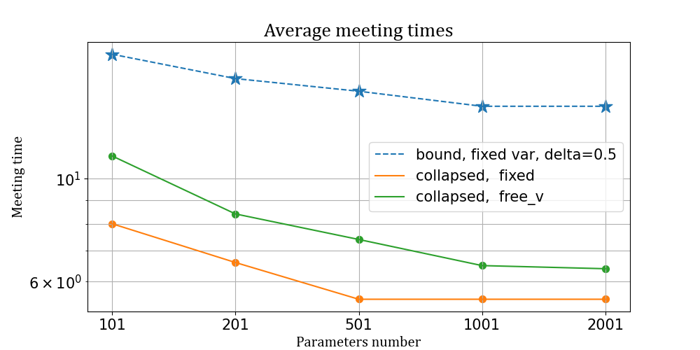
We consider two asymptotic regimes, called outfill asymptotic, where both the number of parameters \(p\) and the number of observation \(N\) increase, but with different speeds according to the chosen setting. Consider first a model with \(K=2\) factors and \(I_1= I_2 = \{50, 100,250,500,750,1000 \}\) different possible levels. Suppose that the number of observations grows quadratically wrt the number of parameters, i.e. \[ N= O(p^2)\] \[ p \rightarrow +\infty.\] Below we report the average meeting time for the sampler with fixed and free variances, alongside with the bound for the collapsed Gibbs sampler with fixed variances, for different values of \(I\).
Average meeting times for Gaussian CREMS
Results of the simulations suggest that the expected number of iterations converges to \(O(1)\) as \(N\) increases, while diverges for the plain vanilla Gibbs sampler (not even plotted because of different scale). It is also clear that the bound closely resembles the estimated average meeting times.
We consider now an even sparser asymptotic regime, where instead the number of observation grows at the same rate of the number of parameters.
\[ \frac{N}{p} \approx \alpha \] \[ p \rightarrow +\infty.\] Estimates for the mean number of iterations for the fixed and free variance case are plotted below, alongside the corresponding theoretical bounds.
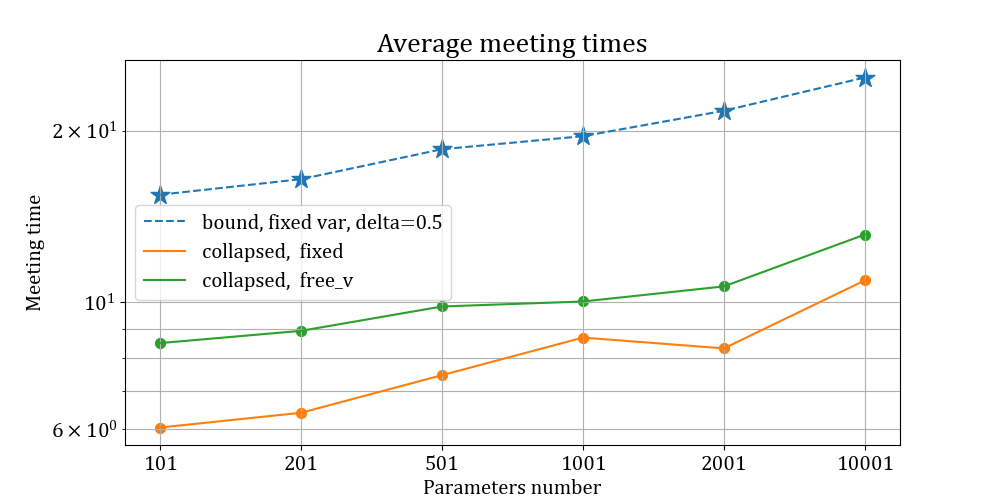
Average meeting times for Gaussian CREMS
Lastly, we want to highlight that while the bound presented in the Theorem above only applies for Gibbs samplers targeting Gaussian distributions, the methodology is still valid for general target distributions and provide small meeting times. We report below the average meeting times of chains targeting a CREM with Laplace response.
\[\begin{equation} \mathcal{L}(y_n) = Laplace \left(\mu +\sum_{k=1}^K a_{i_{k[n]}}^{(k)} \right) \text{ for } n=1,...,N, \end{equation}\]
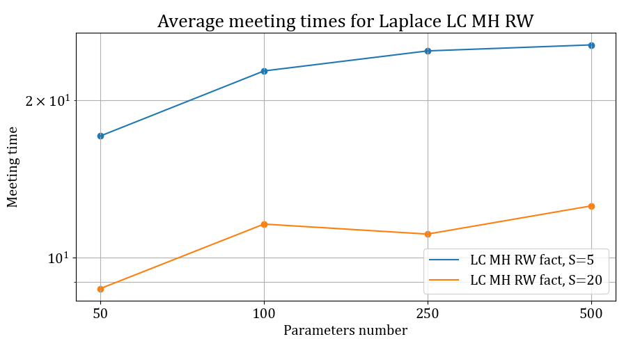
Average meeting times for Laplace CREMS