Overview
In many real data applications we are often required to model jointly \(d\geq 3\) continuous random variables, denoted as \(Y_1,\dots,Y_d\) . The multivariate distribution, which allows us to describe the joint behaviour of those variables, can be denoted as \(F(Y_1,\dots,Y_d)=P(Y_1\le y_1,\dots,Y_d,\le y_d)\) . However, complex relations between data, particularly asymmetric and tail dependent associations, are often difficult to be modelled. The copula approach allows us to express the multivariate distribution of a set of variables by separating the marginals from the dependence structure. Furthermore, the idea of modelling the effect of covariates on the dependence structure described by copulas has recently attracted increasing attention.
Proposal
In Barone and Dalla Valle (2023) we provide a flexible Bayesian mixture model that returns easy-to-interpret results, estimating the effects of covariates on high-dimensional dependence structures and showing good performances in both clustering with unknown number of components and density estimation.
Dirichlet process mixture of conditional vines
Let us consider \(Y_1, \ldots, Y_d\) , which are continuous random variables of interest and let \(\textbf{X}=(X_1, \ldots, X_p)\) be a vector of covariates that may affect the dependence between \(Y_1, \ldots, Y_d\). Then, the conditional joint distribution function of \((Y_1, \ldots, Y_d)\) given \(\textbf{X}= \textbf{x}\) is
\[ F_x (y_1, \ldots, y_d) = P(Y_1 \leq y_1, \ldots, Y_d \leq y_d | \textbf{X}= \textbf{x}), \]
under the assumption that such conditional distribution exists (see Gijbels et al. (2012), Abegaz, Gijbels, and Veraverbeke (2012) and Acar, Craiu, and Yao (2011) ). We denote the conditional marginals of \(F_x\) as
\[ \begin{eqnarray*}F_{1,x}(y_1) & = & P(Y_1 \leq y_1 | \textbf{X}= \textbf{x}), \\& & \ldots \\F_{d,x}(y_d) & = & P(Y_d \leq y_d | \textbf{X}= \textbf{x}). \end{eqnarray*} \]
If the marginals are continuous, then Sklar’s theorem (Sklar 1959) allows us to write
\[ C_x (u_1, \ldots, u_d) = F_x \left( F_{1,x}^{-1} (u_1), \ldots, F_{d,x}^{-1} (u_d) \right) \]
where \(F_{j,x}^{-1} (u_j) = \inf \left\{ y_j : F_{j,x} \geq u_j \right\}\), for \(j = 1,\ldots, d\) , are the conditional quantile functions and \(u_j = F_{j,x}(y_j)\). The conditional copula \(C_x\) fully describes the conditional dependence structure of \((Y_1, \ldots, Y_d)\) given \(\textbf{X}= \textbf{x}\). Therefore, the conditional joint distribution function can be written as
\[ F_x (Y_1, \ldots, Y_d) = C_x \left( F_{1,x}(y_1), \ldots, F_{d,x} (y_d) \right). \]
Let us denote the copula density corresponding to the distribution \(C_x \left( F_{1x}(y_1), \ldots, F_{dx} (y_d) \right)\) as
\[ c_x \left(u_1, \ldots, u_d \right) = c_{\boldsymbol{\theta}} (u_1, \ldots, u_d | \textbf{x}) = c_{\boldsymbol{\theta}(\textbf{x})} (u_1, \ldots, u_d), \] where \(\boldsymbol{\theta}\) is the parameter vector of the \(d\)-variate copula density. We assume that the function \(\boldsymbol{\theta}(\textbf{x})\) depends on a vector of parameters \(\boldsymbol{\beta}\) such that \[\begin{equation} \label{condcop} c_{\boldsymbol{\theta}(\textbf{x})} (u_1, \ldots, u_d) = c_{\boldsymbol{\theta}(\textbf{x}| \boldsymbol{\beta})} (u_1, \ldots, u_d) = c_{1:d} (u_1, \ldots, u_d \, | \, \boldsymbol{\theta}(\textbf{x}| \boldsymbol{\beta})). \end{equation}\]
The \eqref{condcop} can be written in terms of vines Czado (2019), where each pair-copula depends on the vector of covariates \(\textbf{X}\).

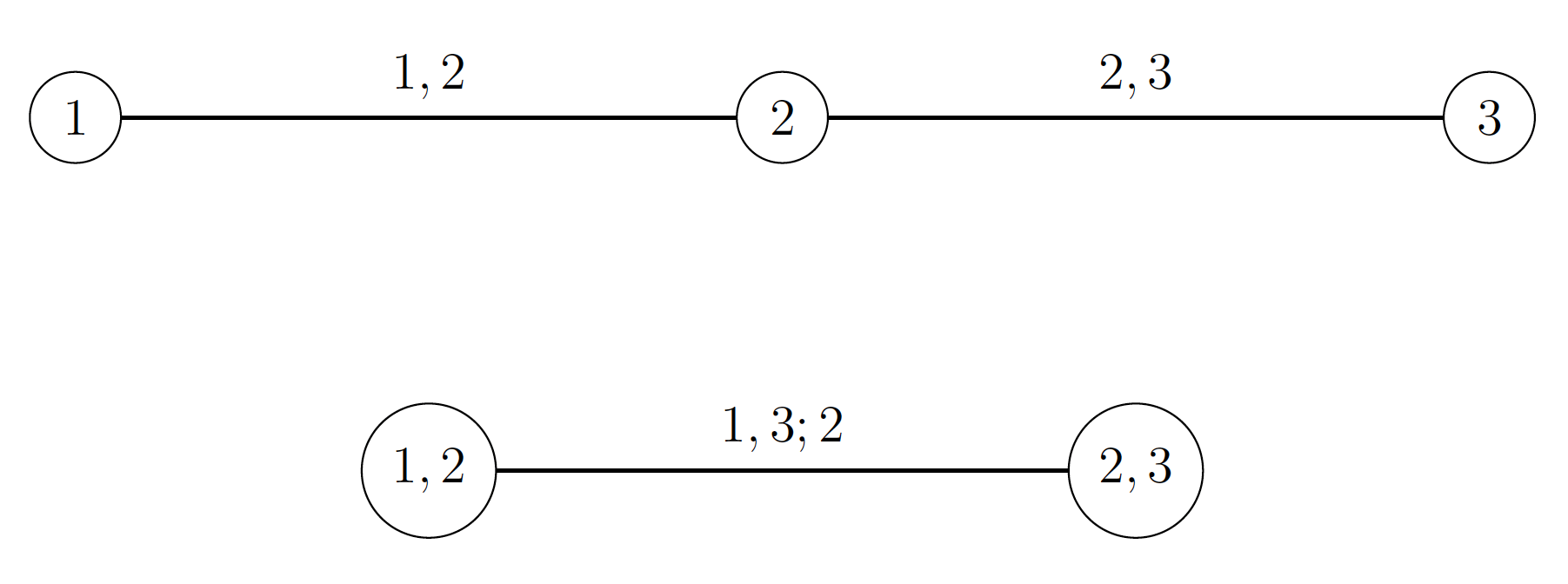
Trivariate vine representation.
The vine representation can be generalized to special vine distribution classes, the most popular of which are D-vines (see Bedford and Cooke (2001), Aas et al. (2009) and Czado (2019)).The conditional D-vine decomposition takes the form
\[ \begin{multline*}c_{1:d} (u_1,\ldots, u_d \,| \,\boldsymbol{\theta}(\textbf{x}| \boldsymbol{\beta})) = \\ \prod_{\ell=1}^{d-1}\prod_{k=1}^{d-\ell}c_{k,\ell+k; k+1, \ldots, k+\ell-1}\left\{F_{k | k+1, \ldots, k+\ell-1,x} (y_k | y_{k+1, \ldots, k+\ell-1}), \right. \\ \left. F_{\ell+k | k+1, \ldots, k+\ell-1,x} (y_{\ell+k}| y_{k+1, \ldots, k+\ell-1}) \, | \, \boldsymbol{\theta}_{k,\ell+k; k+1, \ldots, k+\ell-1}(\textbf{x}| \boldsymbol{\beta})\right\}.\end{multline*} \]
In Barone and Dalla Valle (2023), we model multivariate dependence structures specified as the product of \(\nu=d(d-1)/2\) pair copulas, indexed by the \(\nu\times(q+1)\)-dimensional vector of parameters \(\boldsymbol{\beta}\). The covariates \(f_{h}(x_h)\), \(h=1,\dots,p\), are independent random variables with parameters \(\boldsymbol{\phi}=\left (\phi_{1},\dots,\phi_p \right)\). Note that \(q\ge p\) and its value depends on the chosen link function; for example if the link is linear \(q=p\). Let the vector of parameters \(\boldsymbol{\xi}=\left (\boldsymbol{\beta},\boldsymbol{\phi} \right)\) be defined on the parameter space \(\Xi\). We rewrite the density \(\textbf{f}_{G}(\textbf{x}) \cdot c_G(\cdot, \ldots, \cdot | \textbf{x})\) as an infinite mixture of conditional vine copulas with kernel \(\textbf{f}_{\boldsymbol{\xi}}(\textbf{x})\cdot c_{\boldsymbol{\xi}}(\cdot, \ldots, \cdot | \textbf{x})\) with respect to the mixing measure \(G\), that is\[ \textbf{f}_{G} (\textbf{x}) c_{G} (u_1, \ldots, u_d | \textbf{x}) = \int \textbf{f}_{\boldsymbol{\phi_j}}(\textbf{x}) c_{1:d}(u_1, \ldots, u_d \, | \, \boldsymbol{\theta}(\textbf{x} | \boldsymbol{\beta}_j))dG(\boldsymbol{\xi}). \]With a Dirichlet Process (DP) prior on \(G\), we get a Dirichlet Process Mixture (DPM) of conditional vine copulas, which may be alternatively represented as
\[ \textbf{f}_{\boldsymbol{\phi}} (\textbf{x}) c_{ \boldsymbol{\theta}(\textbf{x} | \boldsymbol{\beta}) } (u_1, \ldots, u_d \, | \, \textbf{x}) = \sum_{j=1}^{\infty} \omega_j \,\textbf{f}_{\boldsymbol{\phi_j}}(\textbf{x}) c_{1:d}(u_1, \ldots, u_d \, | \, \boldsymbol{\theta}(\textbf{x} | \boldsymbol{\beta}_j)), \]
where the weights \(\omega_j\) sum to \(1\). The posterior distribution \(\Pi(G| \textbf{Y},\textbf{X})\) is a mixture of DP models, mixing with respect to the latent variables \(\boldsymbol{\xi}_i\) specific to each observation \(i\) \((F_1(y_{1i}),\dots,F_d(y_{di}))\)
for \(i=1,\dots,N\):
\[ G| \textbf{Y},\textbf{X} \sim\int DP\left (MG_0+\sum_{i=1}^N\delta_{\boldsymbol{\phi}_i\boldsymbol{\beta}_i } \right )d\Pi(\boldsymbol{\phi},\boldsymbol{\beta}|\textbf{y},\textbf{x}), \]where \(M\) is the concentration parameter, \(G_0\) is the centring measure and \(\delta_t\) denotes the Dirac measure at \(t\).
Posterior inference is performed via MCMC sampling by using a Pólya-urn scheme for integrating out of the model the random distribution function from the Dirichlet process MacEachern and Müller (1998).
Financial development and natural disasters data
We present an application to a heterogeneous dataset to study the impacts of worldwide natural disasters on international financial development. We define a \(4\)-dimensional vine copula with marginals denoting the FD index in \(4\) consecutive years and consider the occurrence of a natural disaster as a binary covariate taking value \(1\) if the total damage is over 100 million dollars and \(0\) otherwise. The pair copulas parameters are associated to the covariates through a link function \(g\), such that
\[ \rho (\textbf{x} | \boldsymbol{\beta}) = g^{-1} ( \eta(\textbf{x} | \boldsymbol{\beta}) ) \] where \(g^{-1}\) is the Fisher’s transform and \(\eta(\cdot)\) is the calibration function \(\eta=\beta_0 +\beta_1 X\). We set \(M=1\) and \(G_0\) as a flat multivariate Gaussian distribution centred on a vector of zeros.

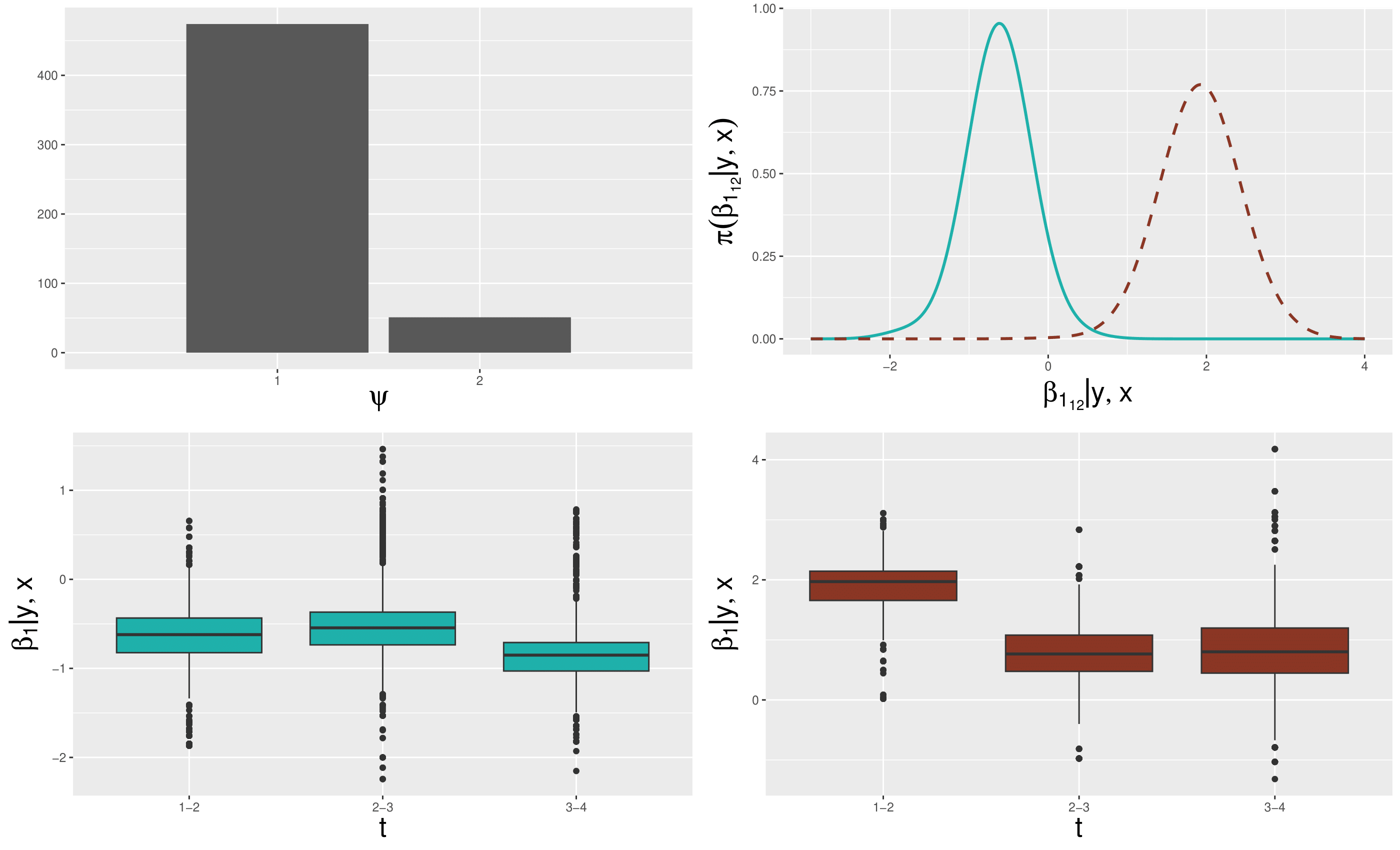
The top left panel shows the barplot of the number of observations allocated to the two estimated mixture components. The top right panel compares the posterior densities of the calibration function parameter \(\beta_{1_{12}}\) (which is related to the first time interval (12)) for the first (solid line) and the second (dashed line) mixture components. The left and right bottom panels show, for the first and second mixture components, the boxplots of the calibration function parameters \(\beta_{1}\) for the first, second and third time intervals (12; 23; 34).
The two estimated mixture components present substantial differences in terms of how they are impacted by natural disasters. For the first cluster (\(\psi=1\)) the model estimates a general negative effect which tends to remain constant until the fourth year; instead, for the second cluster (\(\psi=2\)) the model estimates a positive effect of the natural disaster on the time dependence between yearly FD indexes.
Take home message
In Barone and Dalla Valle (2023) we present an innovative methodology that allows for:
flexible modeling of high-dimensional dependency structures, also considering the impact of one or more covariates and accounting for individual as well as temporal heterogeneity in a natural way;
clustering without assuming the number of components a priori and density estimation;
easy interpretation of the results.