Rough Volatility
New insights about the regularity of the instantaneous variance obtained from realized variance data (see Gatheral, Jaisson, and Rosenbaum (2018), Bennedsen, Lunde, and Pakkanen (2021, to appear) and Fukasawa, Takabatake, and Westphal (2019)), have inspired the development of so-called rough stochastic volatility models in the financial literature. In simple terms, such a model can be described by the following SDE \[\begin{equation} \label{eq:stoch-vol} dS_t = S_t \sqrt{v_t}dB_t, \end{equation}\] where the logarithm of the instantaneous variance process \(v\) behaves similarly to a fractional Brownian motion (fBm) with Hurst index \(0 < H < 1/2\). One of the attractive features of rough volatility models is that they can explain the long-established power-law explosion of the at-the-money (ATM) skew of options as time-to-maturity \(T \to 0\) and, thus, provide excellent fits to the implied volatility surface, as was observed in Bayer, Friz, and Gatheral (2016), but already anticipated much earlier in Alòs, León, and Vives (2007), Fukasawa (2011). In mathematical terms, let \(\sigma_{BS}(T,k)\) denote the implied volatility of an option with time to maturity \(T\) and log-moneyness \(k\). We define the ATM skew as \[\begin{equation*} \text{ATM-skew}(T) = \partial_k \sigma_{BS}(T,k)|_{k=0}, \end{equation*}\] and it is this quantity which can be observed to have a power law explosion when \(T\rightarrow 0\).
Rough volatility models provide a framework which allows to get excellent fits to market data simultaneously w.r.t. to time series of prices of the underlying and to option prices, with few parameters.
Super rough volatility?
Empirical studies of realized variance data as well as studies of the ATM skew in the implied volatility surfaces tend to conclude that \(H \ll 1/2\), often even \(H < 0.1\). As both these estimates involve a certain kind of smoothing – realized variance being an estimate of \(\int_t^{t+h} v_sds\) rather than \(v_t\) itself, option prices and their implied skews being in general not available or reliably very close to maturity – this begs the question, if \(H\) actually might even be equal to \(0\).
From the realized variance viewpoint, Fukasawa, Takabatake, and Westphal (2019) indeed seems to suggest that \(H\) could be \(0\). However, for a fractional Brownian motion, \(H=0\) is not allowed since in this case the integral kernel of the fractional Brownian motion is no longer square integrable, and thus new processes or techniques must be employed in order to study the behavior of stochastic volatility models in this regime. Some interesting efforts has been made to understand this problem. In particular, the theory of Gaussian multiplicative chaos has been used to this end, see for instance the review paper Rhodes and Vargas (2014). Indeed, a proper scaling limit of fBm \(W^H\) as \(H \to 0\) produces a log-correlated Gaussian field (see, for instance, Neuman and Rosenbaum (2018) and Hager and Neuman (2020)). However, the resulting random element is no longer a (continuous) stochastic process and only makes sense in terms of a generalized function (distribution), and it is therefore more challenging to use in practice.
Logarithmic modulation of the fBm
In our recent work Bayer, Harang, and Pigato (2021) we investigate the \(H=0\) problem from a different point of view. We consider an actual continuous stochastic process with \(H=0\) by introducing a logarithmic term in the definition of the kernel \(K:\mathbb{R}_+\rightarrow \mathbb{R}\), which for small \(r>0\) behaves similarly to \[\begin{align} r^{H-\frac{1}{2}}\log(1/r)^{-p}\label{eq1}\tag{1} \end{align}\] for some parameter \(p>1\). This modification ensures that \(K\) remains square integrable for all \(H \in [0,1/2)\). Hence, the resulting family of Gaussian Volterra processes \(\hat{W}\) will be continuous and with finite variance even for \(H=0\), and the ambiguities of the asymptotic analysis for \(H\to0\) cease to matter, as we can simply do the asymptotic for \(H=0\). We stress again that \(\hat{W}\) is a proper, continuous Gaussian process even for \(H=0\).
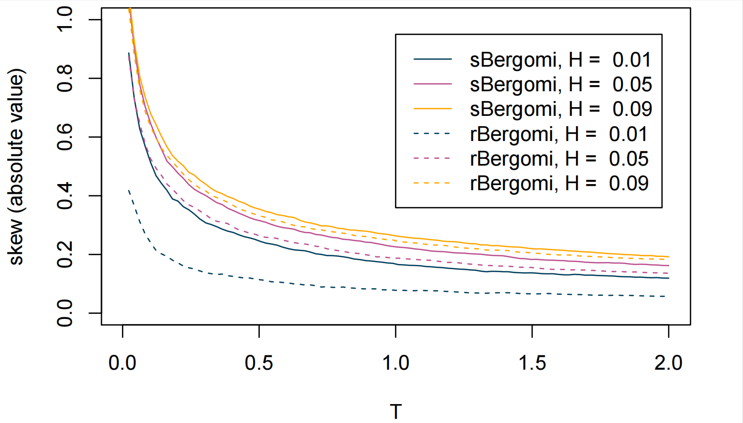
At the same time, as we apply our logarithmic modification only close to the singularity of the power-law kernel, we may expect that the resulting rough volatility models are close to the corresponding standard rough volatility models for \(H \gg 0\), see Figure 1 where we compare the classical rough Bergomi model with the so called super rough Bergomi model (created with the logarithmic modification of the fBm).
Above: Comparisons between the ATM skews of a rough Bergomi model and a corresponding super-rough Bergomi model for \(H \in \{0.01, 0.05, 0.09\}\). Skews are computed by Monte Carlo simulation.
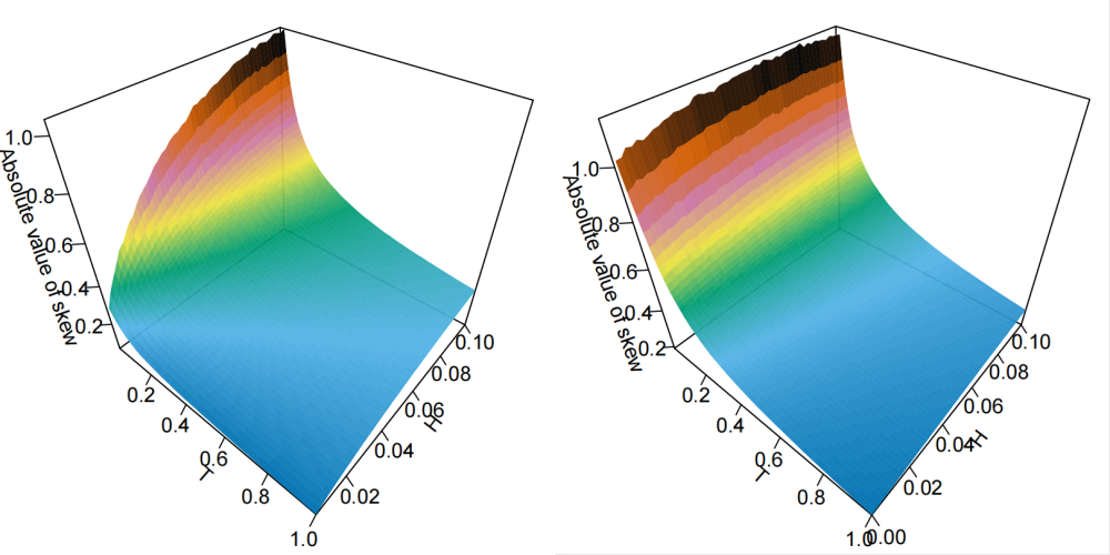
Above: ATM implied volatility skews (absolute values) in the (super-) rough Bergomi model plotted against expiry \(t\) and Hurst index \(H\). Skews are computed by Monte Carlo simulation based on exact simulation of the underlying (log-modulated) fBm. Note that \(H = 0\) is included in the plot in the super-rough case. Note how this seems in keeping with the findings in Forde et al. (2020), of a vanishing skewness as \(H\downarrow 0\) in rough Bergomi.
The power law explosion of the ATM skew
The process we propose here can be seen as an extension of the log Brownian motion studied in Mocioalca and Viens (2005), to include a fractional power. This allows for a better comparison with classical fractional processes, such as the Riemann-Liouville fractional Brownian motion, typically used in rough volatility models.
In this way, we are able to obtain rough volatility models which allow continuous interpolation for \(H \in [0,1/2)\), in the sense that all such choices of \(H\) are valid within the same model, with no apparent breaks between them. To illustrate this observation, we consider a super-rough Bergomi model, which is simply obtained by replacing the Riemann-Liouville fBm by the process \(\hat{W}\) in the rough Bergomi model of Bayer, Friz, and Gatheral (2016). Figure 2 shows the ATM-skew for various expires and values of \(H\) between – and including – \(0\) and \(0.1\). Indeed, the surface “looks” smooth in \(H\), visually indicating a smooth transition from the power law explosion \(T^{H-1/2}\) for \(H>0\) to the skew behaviour at \(H = 0\).
In contrast, the skew-behaviour changes remarkably for the standard rough Bergomi model for small \(H\), see Figure 1. In particular, the skew flattens significantly for very small \(H\). The log-modulated version in Figure 2 shows no signs of this flattening. To the contrary, a more refined analysis, which is the main goal of our article, shows that the skew behaves like \(T^{H-1/2}\) – up to logarithmic terms – and, hence, steepens as \(H \to 0\).
Note in particular that the log-fBm does not have a scale invariance property due to the logarithmic term in the kernel, thereby making any short time asymptotics very difficult. However, by employing the vol-of-vol expansion in Fukasawa (2011) we obtain an asymptotic formula for the ATM skew when the volatility-of-volatility \(\epsilon\) is small. Indeed, we obtain a skew formula of the form \[\begin{equation} \label{eq:skew-asymptotic} \text{ATM-skew} \approx a_{H,\zeta,p}\, \rho \,\log(1/T)^{-p} \, T^{H-1/2} \epsilon, \text{ as } T \to 0, \end{equation}\] with Hurst parameter \(H\in[0,1/2)\), see Theorem 5.4 in Bayer, Harang, and Pigato (2021). Here, \(p>1\) is a parameter of the kernel defined in \(\eqref{eq1}\), and \(a_{H,\zeta,p}\) is a constant depending on \(H\) – and other parameters – which is smooth in \(H\) with \(a_{0,\zeta,p} \neq 0\). This shows us that the explosion of the ATM skew in a stochastic volatility model generated from the log modulated version of a fBm behaves similarly to \(T^{H-\frac{1}{2}}\), the power law explosion of the rough Bergomi model when \(H>0\), while still preserving this property when \(H=0\), providing a simple extension of the rough Bergomi model to capture an important feature of the volatility surface.
Disclaimer: The following material is based on the published article Bayer, Harang, and Pigato (2021), and the reuse of figures and material for the blog post has been approved by the journal SIAM Journal of Financial Mathematics.