Procrustes Analysis for High-Dimensional Data

Background

Let \(\{\mathbf{X}_{i} \in \mathrm{I\!R}^{n \times m} \}_{i = 1,\dots ,N}\) be a set of matrices to be aligned and \({\mathcal {O}}(m)\) the orthogonal group in dimension \(m\). The perturbation model is defined as

\[\begin{equation} {\mathbf{X}}_i= \alpha _i ({\mathbf{M}} + {\mathbf{E}}_i){\mathbf{R}}_i^\top + {\mathbf {1}}_n^\top {\mathbf{t}}_i \quad \quad \text {subject to }\quad {\mathbf{R}}_i \in {\mathcal {O}}(m) \end{equation}\]

where \({\mathbf{E}}_i \sim \mathcal{MN}\mathcal{}_{n,m}(0,\mathbf{\Sigma }_n,\mathbf{\Sigma }_m)\) - i.e., the matrix normal distribution with \(\mathbf{\Sigma }_n \in \mathrm{I\!R}^{n \times n}\) and \(\mathbf{\Sigma }_m \in \mathrm{I\!R}^{m \times m}\) scale parameters - \({\mathbf{M}} \in \mathrm{I\!R}^{n \times m}\) is the shared reference matrix, \(\alpha_i \in \mathrm{I\!R}^{+}\) is the isotropic scaling, \(\mathbf{t}_i \in \mathrm{I\!R}^{1 \times m}\) defines the translation vector, and \({\mathbf{1}}_n \in \mathrm{I\!R}^{1 \times n}\) is a vector of ones.

This work mainly aims to compare the shapes \(\mathbf{X}_{i}\) instead of the form’s analysis of the matrices. For that, the parameters of interest are \(\mathbf{R}_i\), \(\alpha_i\) and \(\mathbf{t}_i\), whereas \(\mathbf{M}\), \(\mathbf{\Sigma}_n\), and \(\mathbf{\Sigma}_m\) are considered as nuisance parameters for each \(i=1,\dots,N\). Clearly, the estimation of the unknown parameters changes if these nuisance parameters are

• Known (Theorem 1 in Andreella and Finos, 2022): Let the SVD of \({\mathbf{X}}_i^\top \mathbf{\Sigma }_n^{-1} {\mathbf{M}} \mathbf{\Sigma }_m^{-1}\) be \({\mathbf{U}}_i {\mathbf{D}}_i {\mathbf{V}}_i^\top\). Then, the maximum likelihood estimators equal \[\begin{equation} \hat{\mathbf{R}}_i^\top = {\mathbf{U}}_i {\mathbf{V}}_i^\top \quad \hat{\alpha _i}_{\hat{\mathbf{R}}_i^\top}^{\top}=||\mathbf{\Sigma }_m^{-1/2}\hat{\mathbf{R}}_i^\top {\mathbf{X}}_i^\top \mathbf{\Sigma }_n^{-1/2}||^2/tr({\mathbf{D}}_i). \tag{1} \end{equation}\]

• Unknown (Algorithm 1 in Andreella and Finos, 2022): no closed-form solution for \(\mathbf{R}_i\) and \(\alpha_i\), and an iterative algorithm proposed by Gower, 1975 must be used where at each step the nuisance parameters are updated.

When \(n<<m\) in both cases (unknown and known nuisance parameters) the Procrustes solutions are infinite (Lemma 1 in Andreella and Finos, 2022) and the SVD leads to polynomial time complexity in \(m\), i.e., we must deal with problems (i) and (ii) described in the first section.

ProMises model and Efficient ProMises model

In Andreella and Finos, 2022, we dealt with problem (i) proposing the ProMises (Procrustes von Mises–Fisher) model, while with problem (ii) proposing the Efficient ProMises model. Therefore:

1. The ill-posed problem is solved by assuming that the orthogonal matrix parameter \(\mathbf{R}_i\) follows the von Mises–Fisher distribution (Downs, 1972), i.e.,\[f({\mathbf{R}}_i) = C({\mathbf{F}}, k ) \exp \big \{tr(k {\mathbf{F}}^\top {\mathbf{R}}_i)\big \},\] and choosing a proper location matrix parameter \(\mathbf{F} \in \mathbb{R}^{m \times m}\). We call this extension the ProMises model. In particular, \(\mathbf{F} \in \mathbb{R}^{m \times m}\) must be specified to be a full rank matrix to have a unique maximum a posteriori solution for \(\mathbf{R}_i\) with the orientation structure of \(\mathbf{F}\) (Lemma 3 in Andreella and Finos, 2022). The prior information about \({\mathbf{R}}_i\)’s structure is directly entered in the SVD step; the maximum a posteriori estimators turn out to be a slight modification of the estimators defined in Equation (1). We decompose \({\mathbf{X}}_i^\top \mathbf{\Sigma }_n^{-1} {\mathbf{M}} \mathbf{\Sigma }_m^{-1} + k {\mathbf{F}}\) instead of \({\mathbf{X}}_i^\top \mathbf{\Sigma }_n^{-1} {\mathbf{M}} \mathbf{\Sigma }_m^{-1}\) (Theorem 2 in Andreella and Finos, 2022).

2. The computational burden is reduced, proving that the minimization problem is solved by projecting the matrices \(\mathbf{X}_i\) into an \(n\)-lower dimensional space using a specific semi-orthogonal transformation. Considering the thin SVD of \({\mathbf{X}}_i = {\mathbf{L}}_i {\mathbf{S}}_i {\mathbf{Q}}_i^\top\) for each \(i=1\dots,N\), where \(\mathbf{Q}_i\) has dimensions \(m \times n\), the following holds \[\max _{{\mathbf{R}}_i \in {\mathcal {O}}(m)} tr({\mathbf{R}}_i^\top {\mathbf{X}}_i^\top \mathbf{\Sigma }_n^{-1} {\mathbf{X}}_j \mathbf{\Sigma }_m^{-1} + k \mathbf{F}) = \max _{{\mathbf{R}}_i^{\star } \in {\mathcal {O}}(n)} tr({\mathbf{R}}_i^{ \star \top } {\mathbf{Q}}_i^\top {\mathbf{X}}_i^\top \mathbf{\Sigma }_n^{-1} {\mathbf{X}}_j \mathbf{\Sigma }_m^{-1} {\mathbf{Q}}_j^\top + k \mathbf{Q}_i^\top \mathbf{F} \mathbf{Q}_j)\] (Lemma 5 in Andreella and Finos, 2022). We reach the same maximum while working in the reduced space of the first \(n\) eigenvectors, which contains all the information, instead of the full data set. The ProMises model applies to matrices with virtually any number of columns. We denote this approach as the Efficient ProMises model. In practice, it projects the matrices \(\mathbf{X}_i\) into an \(n\)-lower-dimensional space using a specific semi-orthogonal transformation \(\mathbf{Q}_i\) which preserves all the data’s information. It aligns, then, the reduced \(n \times n\) matrices \(\{{\mathbf{X}}_i {\mathbf{Q}}_i \in \mathrm{I\!R}^{n \times n }\}_{i = 1, \dots , N}\) by the ProMises model. Finally, it projects the aligned matrices back to the original \(n \times m\)-size matrices \(\{{\mathbf{X}}_i \in \mathrm{I\!R}^{n \times m }\}_{i = 1, \dots , N}\) using the transpose of \(\{{\mathbf{Q}}_i\}_{i = 1, \dots , N}\).

Finally, we proved that the proposed prior distribution is conjugate, making the estimation process quite fast (Algorithm 2 in Andreella and Finos, 2022). The location posterior parameter equaling the following:

\[{\mathbf{F}}^\star =\mathbf{X_i}^\top \mathbf{\Sigma }_n^{-1} {\mathbf{M}} \mathbf{\Sigma }_m^{-1} + k {\mathbf{F}}.\]

which can be rephrased as a combination of the maximum likelihood estimate \(\mathbf{{\hat{R}}}_i\) and the prior mode \(\mathbf{P}\) (i.e., the orthogonal part of \(\mathbf{F}\)), multiplied by corresponding measures of variation.

The method proposed is implemented in https://github.com/angeella/ProMisesModel using the programming language Python and in https://github.com/angeella/alignProMises in the R package alignProMises.

Motivation

The alignment problem is recognized in fMRI multi-subject studies because the brain’s anatomical and functional structures vary across subjects. The most used anatomical alignment is the Montréal Neurological Institute (MNI) space normalization, i.e., the brain images are aligned to an anatomical template by affine transformations using a set of major anatomical landmarks. However, this alignment does not explore the between-subjects variability in anatomical positions of the functional loci since the functional brain regions are not consistently placed on the anatomical landmarks defined by the MNI template.

Specifically, each subject’s brain activation can be represented by a matrix, where the rows represent the stimuli/time points, and the columns represent the voxels. The stimuli are time-synchronized among subjects, so we have correspondence among the matrices’ rows. However, the columns are not assumed to be in correspondence among subjects. Each time series of brain activation (i.e., each of the matrices’ columns) represents the voxels’ functional characteristics that the anatomical normalization fails to align. We aim to represent the neural responses to stimuli in a common high-dimensional space rather than in a canonical anatomical space that does not consider the variability of functional topographies loci. For further details about the functional alignment problem in the fMRI data analysis framework, please see Andreella et al. (2022).

Data description

We applied the proposed method to data from Pernet et al. (2015), available at https://openneuro.org/datasets/ds000158/versions/1.0.0. The study consists of neural activations of \(218\) subjects passively listening to vocal (i.e., speech) and nonvocal sounds. Using a standard processing procedure, we preprocessed the data using the Functional MRI of the Brain Software Library (FSL). Anatomical and functional alignments (based on the Efficient ProMises model) were compared, having images preprocessed in the same way, but in one case, the functional alignment was applied, while in the other case not. For details about the experimental design and data acquisition, please see Pernet et al. (2015).

In the fMRI context, we defined the hyperparameter \(\mathbf{F}\) as a Euclidean similarity matrix using each voxel’s \(3\)D anatomical coordinates. In this way, \(\mathbf{F}\) is a symmetric matrix with ones in the diagonal, which means that voxels with the same spatial location are combined with weights equaling \(1\), and the weights decrease as the voxels to be combined are more spatially distant. This definition also satisfies the requirement to have unique solutions of \(\mathbf{R}_i\), i.e., full-rank matrix (Lemma 3 in Andreella and Finos, 2022).

Functional connectivity

We performed seed-based correlation analysis, which shows the level of functional connectivity between a seed and every voxel in the brain. The analysis process was defined as follows: First, the subject images were aligned using the Efficient ProMises model, then the element-wise arithmetic mean across subjects was calculated, and finally, the functional connectivity analysis was developed on this average matrix.

We considered the frontal pole as seed, being a region with functional diversity. Figure 1 shows the correlation values between the seed and each voxel in the brain using data without functional alignment (top of Figure 1 and with functional alignment using the Efficient ProMises model (bottom of Figure 1). The first evidence is that the functional alignment produces more interpretable maps, where the various regions, such as the superior temporal gyrus, are delineated by marked spatial edges, while the non-aligned map produces more spread regions, hence being less interpretable. It is interesting to evaluate the regions more correlated with the frontal pole, for example, the superior temporal gyrus. This region is associated with the processing of auditory stimuli. The correlation of the superior temporal gyrus with the seed is clear in the bottom part of Figure 1, where functionally aligned images are used.

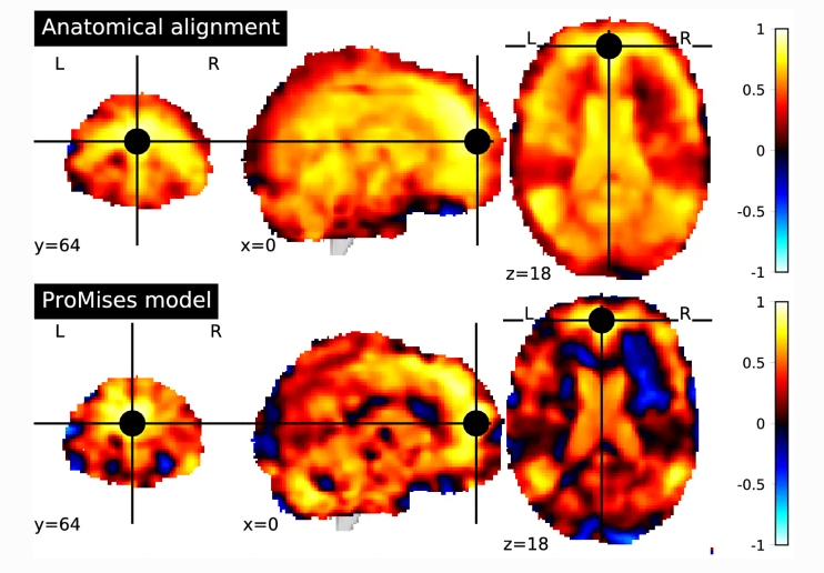
Figure: Seed-based correlation map using data only aligned anatomically (top figure), and data also functionally aligned by the Efficient ProMises model (bottom figure). The black point refers to the seed used (i.e., frontal pole with MNI coordinates (0, 64, 18)).

The preprocessed data are available on the GitHub repository: http://github.com/angeella/fMRIdata, as well as the code used to perform functional connectivity: https://github.com/angeella/ProMisesModel/.

References

Andreella, A., & Finos, L. (2022). Procrustes analysis for high-dimensional data. Psychometrika, 87(4), 1422-1438.
Andreella, A., Finos, L., & Lindquist, M. A. (2023). Enhanced hyperalignment via spatial prior information. Human Brain Mapping, 44(4), 1725-1740.
Downs, T. D. (1972). Orientation statistics. Biometrika, 59(3), 665-676.
Goodall, C. (1991). Procrustes methods in the statistical analysis of shape. Journal of the Royal Statistical Society: Series B (Methodological), 53(2), 285-321.
Gower, J. C. (1975). Generalized procrustes analysis. Psychometrika, 40, 33-51.
Haxby, J. V., Guntupalli, J. S., Connolly, A. C., Halchenko, Y. O., Conroy, B. R., Gobbini, M. I., … & Ramadge, P. J. (2011). A common, high-dimensional model of the representational space in human ventral temporal cortex. Neuron, 72(2), 404-416.
Pernet, C. R., McAleer, P., Latinus, M., Gorgolewski, K. J., Charest, I., Bestelmeyer, P. E., … & Belin, P. (2015). The human voice areas: Spatial organization and inter-individual variability in temporal and extra-temporal cortices. Neuroimage, 119, 164-174.