Overview
Traditionally the excitation noise of spatial and temporal models is Gaussian. Take, for instance, an AR1 (autoregressive of order 1) process, where the increments \(x_{i+1}-\rho x_i, \ \ |\rho|<1\) are assumed to follow a Gaussian distribution. However, it is easy to find datasets that contain inherently non-Gaussian features, such as sudden jumps or spikes, that adversely affect the inferences and predictions made from Gaussian models. In this post, we introduce a specific class of non-Gaussian models, their advantages over Gaussian models, and their Bayesian implementation in Stan and R-INLA, two well-established platforms for statistical modeling.
Why go beyond Gaussian models?
Often, these Gaussian and non-Gaussian models are used as latent components in hierarchical models leading to latent Gaussian models (LGMs) and latent non-Gaussian models (LnGMs), respectively. We highlight next the benefits of using a (latent) non-Gaussian model:
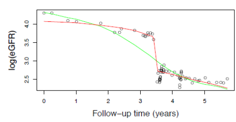
- More accurate predictions. Asar et al. (2020) considered measurements related to the kidney function of several patients recorded over time. The LGM did not adapt well to sudden drops in measurements, as shown in the following figure, which was problematic since these drops are an example of “acute kidney injury”, which should prompt an immediate medical intervention. The red curve shows a prediction based on an LnGM, which clearly is more accurate.
 |
|---|
| Observations of a quantity related to a patient’s kidney function and predictions using an LGM (green) and an LnGM (red). |
Robustness. Non-Gaussian models provide a means for both accommodating possible outliers in the data and reduce their impact on the inferences (West (1984))
Model checking. We often elicit a Gaussian model for simplicity and convenience in a somewhat casual fashion. However, we can fit a non-Gaussian model, and if the relevant inferences do not change significantly, this can confirm the reasonableness of the Gaussian assumption.
What type of non-Gaussian models are you considering?
If \(\mathbf{x}^G\) follows a multivariate Gaussian with mean \(\mathbf{0}\) and precision matrix \(\mathbf{Q}= \mathbf{\mathbf{D}}^T\mathbf{D}\), it can be expressed through
\[ \mathbf{D}\mathbf{x}^G\overset{d}{=} \sigma\mathbf{Z}, \] where \(\mathbf{Z}\) is a vector of i.i.d. standard Gaussian variables. The non-Gaussian extension for \(\mathbf{x}^G\) consists in replacing the driving noise distribution: \[ \mathbf{D}\mathbf{x}\overset{d}{=} \sigma \mathbf{\Lambda}(\eta,\zeta), \] where \(\boldsymbol{\Lambda}\) is a vector of independent and standardized normal-inverse Gaussian (NIG) random variables that depend on the parameter \(\eta\) and \(\zeta\), which controls the leptokurtosis and skewness of the driving noise. Cabral, Bolin, and Rue (2022a) presented these models as flexible extensions of Gaussian models because they contain the Gaussian model as a special case (when \(\eta=0\)), and deviations from the Gaussian model are quantified by the parameters \(\eta\) and \(\zeta\). These models admit a useful variance-mean mixture representation. Considering the mixing variables \(\mathbf{V}= [V_1, \dotsc, V_n]^T\) we have:
\[\begin{align*} \label{eq:model} \tag{1} \mathbf{x}|\mathbf{V} &\sim \text{N}\left(\frac{\sigma}{\sqrt{1+\zeta^2\eta}} \zeta \mathbf{D}^{-1}(\mathbf{V}-\mathbf{1}),\frac{\sigma^2}{1+\zeta^2\eta} \mathbf{D}^{-1}\text{diag}(\mathbf{V})\mathbf{D}^{-T} \right), \ \\ V_{i}|\eta &\overset{ind.}{\sim} \mathrm{IG}(1,\eta^{-1}), \end{align*}\]
where \(\mathrm{IG}\) stands for the inverse-Gaussian distribution. We condition the Gaussian latent field \(\mathbf{x}\) on a vector of mixing variables \(\mathbf{V}\), which enter the covariance matrix, adding more flexibility to the model. We note that the previous parameterization preserves the mean and covariance structure of \(\mathbf{x}\) while allowing for non-zero skewness and excess kurtosis on the marginal distributions.
This non-Gaussian extension can be used in: random walk (RW) and autoregressive processes for time series; simultaneous and conditional autoregressive processes for graphical models and areal data; Matérn processes, which can be used in a variety of applications, such as in geostatistics and spatial point processes. The corresponding dependency matrices \(\mathbf{D}\) that specify each model can be found in Cabral, Bolin, and Rue (2022b).
What sample paths do these models produce?
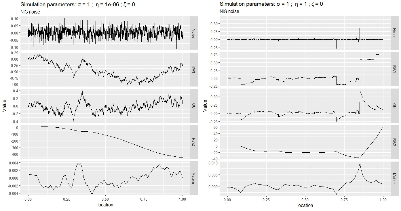
The first row of the following figure shows Gaussian (left) and NIG (right) white noise processes. The rows below show several processes built from these driving noises, including RW1, RW2, Ornstein–Uhlenbeck (OU), and Matérn (\(\alpha=2\)) processes. Whenever the NIG noise takes an extreme value (for instance, near location 0.8), the CRW1 and OU processes will exhibit a distinct jump, and the RW2 and Matérn processes will exhibit a kink (discontinuity in the first derivative).
 |
|---|
| Noise and sample paths of several models for \(\eta=10^{-6}\) (left) and \(\eta=1\) (right), for \(\sigma=1\) and \(\zeta=0\). |
Stan implementation
The Gaussian model (\(\mathbf{D}\mathbf{x}^G = \mathbf{Z}\)) can be declared in Stan as:
x ~ multi_normal_prec(rep_vector(0,N), D'*D)The non-Gaussian model (\(\mathbf{D}\mathbf{x} = \mathbf{\Lambda}\)) declaration is:
x ~ nig_model(D, eta, zeta, h, 1)The argument h should be a vector of ones for discrete-space models. For models defined in continuous space, for instance, a continuous random walk of order 1, h contains the distance between locations. The last argument is an integer with value 1 if the log-determinant of \(\mathbf{D}\) should be computed (if \(\mathbf{D}\) depends on parameters), or 0 otherwise. The nig_model and other Stan functions can be found in github.com/rafaelcabral96/nigstan, along with a more comprehensive theoretical background and several code examples for time series, geostatistical and areal data application. The function nig_model uses a collapsed representation of (1) and leverages within-chain parallelization to improve speed and scalability.
Fitting a non-Gaussian model in Stan (Columbus dataset)
The Columbus dataset consists of crime rates in thousands (\(y_i\)) in 49 counties of Columbus, Ohio, and can be found in the spdep R package. The next Leaflet widget shows the crime rates.
We consider the following model:
\[ y_i= \beta_0 + \beta_1 \text{HV}_i + \beta_2 \text{HI}_i + \sigma\mathbf{x}_i, \] where \(\text{HV}_i\) and \(\text{HI}_i\) are the average household value and household income for county \(i\), and \(\mathbf{x}\) is a simultaneous autoregressive (SAR) model to account for spatially structured random effects. We consider a Gaussian SAR model built from the following relationship:
\[ \mathbf{x} = \mathbf{B}\mathbf{x} + \sigma\mathbf{Z}, \] where each element of the random vector \(\mathbf{x}\) corresponds to a county and \(\mathbf{Z}\) is a vector of i.i.d. standard Gaussian noise. The matrix \(\mathbf{B}\) causes simultaneous autoregressions of each county on its neighbors, where two counties are considered to be neighbors if they share a common border. The diagonal elements of \(\mathbf{B}\) are 0 so each node does not depend on itself. For simplicity, we assume \(\mathbf{B}=\rho\mathbf{W}\), where \(\mathbf{W}\) is a row standardized adjacency matrix and \(-1<\rho<1\) so that the resulting precision matrix is valid. We end up with the system \(\mathbf{D}_{SAR}\mathbf{x} = \sigma\mathbf{Z}\), where \(\mathbf{D}_{SAR}=\mathbf{I}-\rho\mathbf{W}\). The equivalent model driven by NIG noise is then \(\mathbf{D}_{SAR}\mathbf{x} = \sigma\mathbf{\Lambda}\), where \(\mathbf{\Lambda}\) is i.i.d. standardized NIG noise with parameters \(\eta\) and \(\zeta\).
The code for the Stan implementation can be found in this link. Let \(\mathbf{B}\) and \(\mathbf{\beta}=[\beta_0,\beta_1,\beta_2]^T\) stand for the design matrix and the regression coefficients, respectively. Then, the Stan declaration for the Gaussian and non-Gaussian models is as follows:
transformed parameters{
  vector[N] X = (y - B*beta)/sigma;                       // Spatial effects
}

model{

  matrix[N,N] D = add_diag(-rho*W, 1);                    // D = I - rho W;

  //Gaussian model
  //X ~ multi_normal_prec(rep_vector(0,N), D'*D);

  //NIG model
  X ~ nig_model(D, etas, zetas, h, 1);
The posterior mean and standard deviation of the spatial effects can be found on the Leaflet widget. The widget also shows the posterior mean of the mixing variables \(\mathbf{V}\), and from it, we can identify two outlier counties. The posterior distributions of \(\eta\) and \(\zeta\) suggest heavy-tailedness, although no asymmetry, as shown in the following table.
| variable | mean | sd | q5 | q95 | rhat | ess_bulk | ess_tail |
|---|---|---|---|---|---|---|---|
| sigma | 27.41 | 3.34 | 22.10 | 33.10 | 1 | 4578.12 | 5636.57 |
| rho | 0.51 | 0.19 | 0.15 | 0.80 | 1 | 3505.46 | 3361.02 |
| eta | 6.51 | 2.45 | 2.95 | 10.94 | 1 | 5081.12 | 5061.76 |
| zeta | -0.11 | 0.76 | -1.53 | 1.27 | 1 | 1895.06 | 2635.10 |
| beta[0] | 59.30 | 16.32 | 33.02 | 81.45 | 1 | 2091.19 | 2467.55 |
| beta[1] | -0.15 | 0.14 | -0.39 | 0.07 | 1 | 3542.21 | 3231.01 |
| beta[2] | -1.45 | 0.57 | -2.38 | -0.50 | 1 | 2892.18 | 4458.28 |
R-INLA implementation
To account for measurement error, we can consider the following hierarchical model:
\[\begin{equation*} y_i|\mu_i \sim N(\mu_i, \sigma_\epsilon^2), \\ \mu_i = \beta_0 + \beta_1 \text{HV}_i + \beta_2 \text{HI}_i + \sigma\mathbf{x}_i, \end{equation*}\] where \(\sigma_\epsilon^2\) is the measurement error variance, and now the non-Gaussian SAR model \(\mathbf{x}\) is a latent component. When fitting latent models, such as the previous one, the posterior distribution often induces a geometry that frustrates sampling algorithms, such as Stan’s Hamiltonian Monte Carlo (Margossian et al. (2020)).
Recent work on fitting latent non-Gaussian models (LnGMs) using variational Bayes and Laplace approximations permits fast and scalable estimation of these models. The approximation uses R-INLA (Rue, Martino, and Chopin (2009)), and the methods are implemented in the ngvb package (Cabral, Bolin, and Rue (2022b)). The previous latent SAR model is implemented in the ngvb package vignette. There was significant evidence for non-Gaussianity since the Bayes factor between the fitted LGM and LnGM was around 80.000.