Overview
In this post we first review the concept of semi-parametric copula and the accompanying estimation procedure of pseudo-likelihood estimation (PLE). We then generalize the estimation problem to the setting where the copula signal is hidden in a semi- or non-parametric regression model. Under this setting we have to base the PLE on the residuals. The particular challenge of the diverging score function is handled via the technique of the weighted residual empirical processes.
The semi-parametric copula model
Copula has been a popular method to model multivariate dependence structure since its introduction in Sklar (1959). Consider a random vector \(\mathbf{E}=(E_1,\dots,E_p)^\top\in\mathbb{R}^p\) with joint distribution function \(H\); we assume throughout that \(E_k\), \(k\in\{1,\dots,p\}\) has absolutely continuous marginal distribution function \(F_k\). Then the copula \(C\) associated with \(\mathbf{E}\) is the joint distribution function of the marginally transformed random vector \((F_1(E_1),\dots,F_p(E_p))^\top\). It is clear from this definition that \(C\) itself is always a distribution supported on the unit hypercube \([0,1]^p\), and \(C\) always has uniform marginals supported on \([0,1]\) whatever the marginals of \(\mathbf{E}\) may be. (The explicit form of \(C\) follows from the Sklar’s theorem, for instance Corollary 2.10.10 in Nelsen (2006): \(C(\mathbf{u}) = H(F_1^{\leftarrow}(u_1),\dots,F_p^{\leftarrow}(u_p))\) for \(F_k^{\leftarrow}\) the left-continuous inverse of \(F_k\) and \(\mathbf{u} = (u_1,\dots,u_p)^\top\in[0,1]^p\).) Furthermore, by the invariance property, if \(g_1,\dots,g_p\) are univariate strictly increasing functions, then \(\mathbf{E}\) and its marginally transformed version \((g_1(E_1),\dots,g_p(E_p))^\top\) will admit the copula.
Thus, copula is a margin-free measure of multivariate dependence. Applied in the opposite direction, one could also start from a copula and couple the copula with arbitrary marginals to create multivariate distributions in a flexible manner. For instance, beyond the usual applications in finance and economy, copulas could be used in the latter manner to model the dependence among the repeated observations in longitudinal data (Sun, Frees, and Rosenberg (2008)).
In this post we will focus on the semi-parametric copula model that serves as a middle ground between a totally non-parametric approach to copula modelling (via the so called empirical copula, see for instance Fermanian, Radulović, and Wegkamp (2004) and Berghaus, Bücher, and Volgushev (2017)) and a totally parametric modelling of the random vector \(\mathbf{E}\). In the semi-parametric copula model, we consider a collection of possible distributions of \(\mathbf{E}\) where the copulas \(C=C(\mathbf{\cdot};\mathbf{\theta})\) are constrained to be parametrized by an Euclidean copula parameter \(\mathbf{\theta}=(\theta_1,\dots,\theta_d)^\top\), but where the marginals \(F_1,\dots,F_p\) of \(\mathbf{E}\) could range over all \(p\)-tuples of absolutely continuous univariate distribution functions.
The pseudo-likelihood method
In the semi-parametric copula model, the primary interest is often the true value \(\mathbf{\theta}^*\) of the copula parameter that determines the multivariate dependence. An obvious challenge in estimating \(\mathbf{\theta}^*\) in the copula setting is how to handle the unknown marginals \(F_1,\dots,F_p\). The canonical solution is the pseudo-likelihood estimation (PLE) introduced in Oakes (1994) and Genest, Ghoudi, and Rivest (1995) that we now describe.
Let \(g_1(\mathbf{\cdot};\mathbf{\theta}),\dots,g_d(\mathbf{\cdot};\mathbf{\theta})\) be a collection of appropriate score functions such that the population estimating equation \(\mathbb{E} g_m(F_1(E_1),\dots,F_p(E_p);\mathbf{\theta})=0\) holds only when \(\mathbf{\theta}=\mathbf{\theta}^*\), for all \(m\in\{1,\dots,d\}\). In principle one can always choose the score functions to be the ones in the maximum likelihood estimation, namely \(g_m(\cdot;\mathbf{\theta})=\frac{\partial}{\partial \theta_m} \log c(\mathbf{\cdot};\mathbf{\theta})\) where \(c(\mathbf{\cdot};\mathbf{\theta})\) is the density of the copula \(C(\mathbf{\cdot};\mathbf{\theta})\). Thus, if \(F_1,\dots,F_p\) were known, to estimate \(\mathbf{\theta}^*\) empirically based on a sample \(\mathbf{E}_i=(E_{i,1},\dots,E_{i,p})^\top\), \(i\in\{1,\dots,n\}\) of \(\mathbf{E}\), one could simply “find the zero” of the empirical version of the estimating equation, that is to estimate \(\mathbf{\theta}^*\) by \(\mathbf{\hat{\theta}}^{\text{parametric}}\) that solves, for all \(m\in\{1,\dots,d\}\), \[\begin{align*} \frac{1}{n} \sum_{i=1}^n g_m(F_1(E_{i,1}),\dots,F_p(E_{i,p});\hat{\theta}^{\text{parametric}}) =0 . \end{align*}\] (The superscript “parametric” points to the fact that when \(F_1,\dots,F_p\) are known, we are basically solving a parametric problem.) However, in semi-parametric copula modelling we commonly avoid setting \(F_1,\dots,F_p\) to some particular form. The PLE method solves this problem by replacing the unknown \(F_k\), \(k\in\{1,\dots,p\}\) by its empirical counterpart, namely the empirical distribution function \(F_{n,k}(t) = \frac{1}{n+1} \sum_{i=1}^n \mathbf{1}\{E_{i,k} \le t \}\). The oracle PLE estimator \(\mathbf{\hat{\theta}}^{\text{oracle}}\) of \(\mathbf{\theta}^*\) is then the one that solves the following, revised estimating equation: for all \(m\in\{1,\dots,d\}\), \[\begin{align} \frac{1}{n} \sum_{i=1}^n g_m(F_{n,1}(E_{i,1}),\dots,F_{n,p}(E_{i,p});\mathbf{\hat{\theta}}^{\text{oracle}}) = \int g_m(\mathbf{u};\mathbf{\hat{\theta}}^{\text{oracle}})\mathrm{d}C_n(\mathbf{u}) = 0. \label{eq1}\tag{1} \end{align}\] All integrals in this post are over \([0,1]^p\). To simplify our expression above and later, we have introduced the empirical copula \(C_n\) that is a multivariate distribution function on \([0,1]^p\) with a mass of \(1/n\) at each of \((F_{n,1}(E_{i,1}),\dots,F_{n,p}(E_{i,p}))^\top\), \(i\in\{1,\dots,n\}\) (precisely, \(C_n(\mathbf{u}) = \frac{1}{n} \sum_{i=1}^n \mathbf{1}\left\{ F_{n,1}(E_{i,1})\le u_1, \dots, F_{n,p}(E_{i,p})\le u_p \right\}\)). The qualifier “oracle” in \(\mathbf{\hat{\theta}}^{\text{oracle}}\) is used to distinguish the current case when we can still directly observe the copula sample \(\mathbf{E}_i\), \(i\in\{1,\dots,n\}\) (albeit without knowing \(F_1,\dots,F_p\)), from the case when even that sample will be subject to perturbation which we now turn to.
Residual-based pseudo-likelihood for semi-parametric copula adjusted for regression
From now on we suppose that the copula signal \(\mathbf{E}=\mathbf{E}_{\mathbf{\theta}^*}\) is “hidden” in a multivariate response semi- or non-parametric regression model, a setting considered in our recent work (Zhao, Gijbels, and Van Keilegom (2022)): for a covariate \(\mathbf{X}\in\mathbb{R}^q\) (independent of \(\mathbf{E}\)) and a response \(\mathbf{Y}=(Y_1,\dots,Y_p)^\top\in\mathbb{R}^p\), \[\begin{align*} Y_1 &= m_1(\mathbf{X}) + E_1 , \\ &\quad \vdots \\ Y_p &= m_p(\mathbf{X}) + E_p . \end{align*}\] In its raw form, the model above is a purely non-parametric regression model; by specifying particular forms of the regression function \(m_k\), the above will accommodate a wide range of popular non- and semi-parametric regression variants such as the partly linear regression model and the additive model. (It’s not much more difficult to consider a more flexible, heteroscedastic model \(Y_k = m_k(\mathbf{X}) + \sigma_k(\mathbf{X})E_k\), though we refrain from doing so in this post.) Gijbels, Omelka, and Veraverbeke (2015) considered a similar model and studied the resulting empirical copula process.
Under this regression model, we can observe an i.i.d. sample \((\mathbf{Y}_1,\mathbf{X}_1),\dots,(\mathbf{Y}_n,\mathbf{X}_n)\) of \((\mathbf{Y},\mathbf{X})\), but crucially not the copula sample \(\mathbf{E}_1, \dots, \mathbf{E}_n\). To eventually arrive at our estimator for \(\mathbf{\theta}^*\) in this setting, we will first form our empirical copula \(\hat{C}_n\) based on the residuals of the regression as follows. Let \(\hat{m}_k\) be some estimator for \(m_k\). Let’s estimate the \(k\)th component of \(E_i=(E_{i,1},\dots,E_{i,p})^\top\) by the residual \[\begin{align*} \hat{E}_{i,k} = Y_{i,k} - \hat{m}_k(X_i) . \end{align*}\] Then, we form the residual-based empirical distribution and copula: \[\begin{align*} \hat{F}_{n,k}(t) = \dfrac{1}{n+1} \sum_{i=1}^n \mathbf{1}\{ \hat{E}_{i,k} \le t \},\quad \hat{C}_n(\mathbf{u}) = \frac{1}{n} \sum_{i=1}^n \prod_{k=1}^p \mathbf{1}\{\hat{F}_{n,k}(\hat{E}_{i,k})\le u_k \}. \end{align*}\] Finally, to estimate \(\mathbf{\theta}^*\), we settle for the estimator \(\hat{\theta}^{\text{residual}}\) that solves \[\begin{align} \frac{1}{n} \sum_{i=1}^n g_m( \hat{F}_{n,1}(\hat{E}_{i,1}),\dots,\hat{F}_{n,p}(\hat{E}_{i,p}) ;\hat{\theta}^{\text{residual}}) = \int g_m(\mathbf{u};\hat{\theta}^{\text{residual}})\mathrm{d}\hat{C}_n(\mathbf{u}) = 0 . \label{eq2}\tag{2} \end{align}\]
Comparing Eq. (2) to Eq. (1), we would expect that when the residual-based empirical copula \(\hat{C}_n\) is asymptotically indistinguishable from the oracle empirical copula \(C_n\), the residual-based copula parameter estimator \(\hat{\theta}^{\text{residual}}\) should be asymptotically indistinguishable from \(\hat{\theta}^{\text{oracle}}\) as well. To formally reach this conclusion, standard estimating equation theory requires (among other conditions that we will ignore in this post) that the estimating equations at the truth should become indistinguishable, namely \[\begin{align} \int g_m(\mathbf{u};\mathbf{\theta}^*)\mathrm{d}\hat{C}_n(\mathbf{u}) - \int g_m(\mathbf{u};\mathbf{\theta}^*)\mathrm{d}C_n(\mathbf{u}) = o_p(n^{-1/2}) . \label{eq3}\tag{3} \end{align}\]
One typical, although ultimately restrictive, approach to establish Eq. (3) is to invoke integration by parts (Neumeyer, Omelka, and Hudecová (2019), Chen, Huang, and Yi (2021)): ideally, this would yield \[\begin{align*} \int g_m(\mathbf{u};\mathbf{\theta}^*)\mathrm{d}\hat{C}_n(\mathbf{u}) \sim &\int \hat{C}_n(\mathbf{u})\mathrm{d}g_m(\mathbf{u};\mathbf{\theta}^*) \\ \stackrel{\text{up to}~o_p(n^{-1/2})}{\approx} & C_n(\mathbf{u})\mathrm{d}g_m(\mathbf{u};\mathbf{\theta}^*) \sim \int g_m(\mathbf{u};\mathbf{\theta}^*)\mathrm{d}C_n(\mathbf{u}) . \end{align*}\] In the above “\(\sim\)” is only meant to give a drastically simplified and hence not-quite-correct representation of integration by parts (we refer the readers to Appendix A in Radulović, Wegkamp, and Zhao (2017) for a precise multivariate integration by parts formula particularly useful for copulas), but it already conveys the underlying idea: the aim is to convert \(\hat{C}_n\) and \(C_n\) in the integrals from measures to integrands so that proving the closeness between the two integrals is clearly reduced to proving the closeness between \(\hat{C}_n\) and \(C_n\). However, the integration by parts trick, although popular, often requires bounded \(g_m\) to properly define the measure \(\mathrm{d}g_m\), but this is often not satisfied for even the most common copulas. For instance, in Gaussian copula, the score functions are quadratic forms of the \(\Phi^{\leftarrow}(\mathbf{u}_k)\)’s where \(\Phi^{\leftarrow}\) is the standard normal quantile function (see Eq. (2.2) in Segers, Akker, and Werker (2014)), so are clearly divergent as \(u_k\) approaches 0 or 1.
In Zhao, Gijbels, and Van Keilegom (2022) we instead adopted a more direct approach. Let \(g_m^{[k]}(\mathbf{u};\mathbf{\theta}^*)=\frac{\partial}{\partial u_k} g_m(\mathbf{u};\mathbf{\theta}^*)\). Then Taylor-expanding Eq. (3) we see that we will need (among other ingredients) an \(o_p(n^{-1/2})\) rate for the terms on the right-hand side of \[\begin{align} \int g_m(\mathbf{u};\mathbf{\theta}^*)\mathrm{d}({\hat{C}_n-C_n})(\mathbf{u}) \approx \sum_{k=1}^p \left[ \frac{1}{n} \sum_{i=1}^n g_m^{[k]}(F_k(E_{i,k});\mathbf{\theta}^*) \left\{ \hat{F}_{n,k}(\hat{E}_{i,k})-F_{n,k}(E_{i,k}) \right\} \right] . \label{eq4}\tag{4} \end{align}\] It is not enough that the terms \(\hat{F}_{n,k}(\hat{E}_{i,k})-F_{n,k}(E_{i,k})\) on the right-hand side are \(o_p(n^{-1/2})\) (in fact they are not), due to the divergence of \(g_m^{[k]}\). We need to take a more careful look at \(\hat{F}_{n,k}(\hat{E}_{i,k})-F_{n,k}(E_{i,k})\), whose analysis belongs to residual empirical processes. To demonstrate the benefits of considering the weighted version of such processes, we first review some basic literature on the weighted (non-residual) empirical processes in the simplified setting of the real line.
Weighted empirical processes on the real line
In this section we consider estimating a distribution function \(F=F_U\) of a random variable \(U\). We rely on the empirical distribution function \(F_n\) constructed from the i.i.d. observations \(U_1, \dots, U_n\) of \(U\): \(F_n(t) = \frac{1}{n+1} \sum_{i=1}^n \mathbf{1}\left\{U_i\le t\right\}\). The resulting classical empirical process on the real line \(\sqrt{n} (F_n -F)(t)\), \(t\in \mathbb{R}\) must be one of the most extensively studied objects in all of probability; for illustration we will just quote a form of the associated law of the iterated logarithm (LIL): \[\begin{align*} \limsup_{n\rightarrow\infty} \sup_{t} \left|\dfrac{1}{\sqrt{\log\log(n)}} \sqrt{n} (F_n -F)(t) \right| = \dfrac{1}{\sqrt{2}} . \end{align*}\] Clearly, the LIL treats all points \(t\in \mathbb{R}\) equally. However, in reality the \(F(t)\) at some \(t\) is easier to estimate than others. This is essentially because the variability \(\text{var}\left\{F_n(t)\right\}=F(t)\left\{1-F(t)\right\}/n\) approaches \(0\) when \(F(t)\) approaches \(0\) or \(1\), for any \(n\). We can clearly observe this feature in the small simulation study represented by the following figure, where the “band” enclosing the deviations (based on 100 Monte-Carlo simulations) gets narrower toward the boundaries of the support of \(U\).
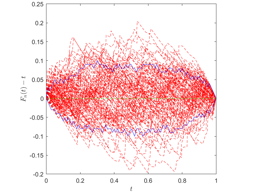
Above: Plot of the deviation \(F_n-F\), for sample size \(n=50\), based on 100 Monte-Carlo simulations. For simplicity we assumed \(U\sim{Unif}(0,1)\), so \(F(t)=t\) for \(t\in[0,1]\). The deviation from each simulation is represented by a single red dashed line. The 10% and 90% quantiles of the deviations at each \(t\) value are indicated by the two blue lines. Clearly, the “band” enclosing the deviations gets narrower toward the boundaries of the support of \(U\).
This feature can also be characterized theoretically. For instance, we can find the LIL for the weighted process \(\sqrt{n}(F_n -F)/\sqrt{F}\), that is the classical process but now scaled by an additional standard deviation factor \(1/\sqrt{F}\), from Csáki (1977): for some \(0<C<\infty\), \[\begin{align*} \limsup_{n\rightarrow\infty} \sup_{F(t)\in(\frac{1}{n},\frac{1}{2}]} \left|\dfrac{\log\log\log(n)}{\log\log(n)} \sqrt{n}\dfrac{(F_n -F)(t)}{\sqrt{F(t)}}\right| = C. \end{align*}\] Compared to the LIL for the unweighted process earlier, we can see that the weighted process is just slightly more difficult to bound, but now \(\sqrt{n}(F_n -F)(t)\) clearly enjoys a tighter bound toward the boundaries of the support of \(U\) due to the vanishing \(\sqrt{F(t)}\) there.
Such results on the weighted empirical processes can be generalized to settings beyond the real line, for instance to sets in \(\mathbb{R}^p\) (Alexander (1987)) and sets of functions (Giné, Koltchinskii, and Wellner (2003)).
Results for residual-based estimators
For us, the idea of the weighted empirical processes will be applied to the residual empirical processes, which will further culminate in our eventual result on the residual-based estimator \(\hat{\theta}^{\text{residual}}\) for the copula parameter. We will first consider the weighted residual empirical processes.
Results on weighted residual empirical process
Let \(f_k\) be the density of \(E_k\), and \(\cal{T}_n\) be the \(\sigma\)-field generated by the \((\mathbf{X}_i,\mathbf{Y}_i)\)’s, \(i\in\{1,\dots,n\}\). The usual decomposition of a residual empirical process is \[\begin{align*} \hat{F}_{n,k}(t) - F_{n,k}(t) = f_k(t) \cdot \mathbb{E}\left[ (\hat{m}_k-m_k)(\mathbf{X}) | \cal{T}_n \right] + r_{1,k}(t) \end{align*}\] where \(r_{1,k}\) is a remainder term that could be controlled as follows:
Theorem: Suppose that we can embed \(\hat{m}_k-m_k\) into a function class \(\cal{D}\) with bracketing number \(N_{[]}(\tau,\cal{D}) \lesssim (1/\tau)^\beta \exp(K (1/\tau)^{1/\nu})\) where \(\beta\), \(K\) and \(\nu\) are constants. Suppose that \(\|\hat{m}_k-m_k\|_\infty=O_p(a_n)\) (where \(\|\cdot\|_\infty\) is the supremum norm over the support of \(\mathbf{X}\)). Then under mild regularity conditions, \[\begin{gather*} \sup_{t\in\ \mathbb{R}} \dfrac{|r_{1,k}(t)|}{ n^{-\frac{1}{2}} \left\{ f_k(t) \cdot a_n + a_n^2\right\}^{\frac{1}{2}(1-1/\nu)} + n^{-\frac{1}{1+1/\nu}} + a_n^2 } = O_p( 1 ) . \end{gather*}\]
Clearly, the convergence rate of the remainder term \(r_{1,k}\) is improved by both the rate of \(\|\hat{m}_k-m_k\|_\infty\) and the weight \(f_k\). The latter point is especially beneficial when \(f_k\) is a density “of the usual shape” that decays at its tails, which will allow the rate of \(r_{1,k}\) to be tightened accordingly (exactly similar to how the rate of \(\sqrt{n}(F_n -F)(t)\) is tightened by \(\sqrt{F(t)}\) in the weighted empirical processes on the real line that we reviewed earlier). These features will tame the divergence of \(g_m^{[k]}\) in Eq. (4).
Because what eventually form the ingredients of the residual-based copula \(\hat{C}_n\) are the residual ranks \(\hat{F}_{n,k}( \hat{E}_{i,k} )\)’s, we need to go one step further and consider the analogous results for them:
Theorem: For all \(n\ge 1\), \(k\in\{1,\dots,p\}\) and \(i\in\{1,\dots,n\}\), \[\begin{align} \label{eq5}\tag{5} \hat{F}_{n,k}( \hat{E}_{i,k} ) - F_{n,k}( E_{i,k} ) &= -f_k(E_{i,k}) \left\{ (\hat{m}_k-m_k)(\mathbf{X}_i) - \mathbb{E}\left[ (\hat{m}_k-m_k)(\mathbf{X}) | \cal{T}_n \right] \right\} + r_{1,k}( \hat{E}_{i,k} ) + r_{2,k,i} \end{align}\] where \(r_{1,k}\) is as in the last theorem, and \(r_{2,k,i}\) is another remainder term that satisfies \[\begin{align*} \max_{i\in\{1,\dots,n\}} \dfrac{ |r_{2,k,i}| }{ \log^{\frac{1}{2}}(n) n^{-\frac{1}{2}} \left\{ f_k(E_{i,k})\cdot a_n \right\}^{\frac{1}{2}} + a_n^2 } = O_p(1) . \end{align*}\]
Note that similar to \(r_{1,k}\) earlier, the rate of \(r_{2,k,i}\) also enjoys the dependence on \(\|\hat{m}_k-m_k\|_\infty\) and the weighing by \(f_k\).
Results on residual-based estimator for the copula parameter
We are now ready to plug in the decomposition of \(\hat{F}_{n,k}( \hat{E}_{i,k} ) - F_{n,k}( E_{i,k} )\) in Eq. (5) in the last theorem into (4). The leading term in Eq. (5) (the one proportional to \(f_k\)), which is centered, is now summed over \(i\in\{1,\dots,n\}\) in (4) and so enjoys an additional \(n^{-1/2}\)-scaling. The remainder terms are weighted and so tame the divergence of the scores \(g_m^{[k]}\). Eventually, we arrive at the asymptotic equivalence between the residual-based PLE and the oracle PLE:
Theorem: Under the conditions of the last two theorems, and some additional regularity conditions which in particular require, for \(m\in\{1,\dots,d\}\) and \(k\in\{1,\dots,p\}\), \[\begin{align} \int \left\{g_m^{[k]}(\mathbf{u};\mathbf{\theta}^*) f_k(F_k^{\leftarrow}(u_k)) \right\}^2\mathrm{d}C(\mathbf{u}) < \infty, \label{eq6}\tag{6} \end{align}\] the asymptotic equivalence in Eq. (3) holds. Furthermore, \(\hat{\theta}^{\text{residual}} - \hat{\theta}^{\text{oracle}} = o_p(n^{-1/2})\).
Condition (6) in fact allows for quite non-trivial divergence of the score functions \(g_m\) (it certainly accommodates the Gaussian and the \(t\)-copulas). To apply the theorem above, one still needs to verify the correct upper bound on the bracketing number for embedding \(\hat{m}_k-m_k\), which again turns out to be non-restrictive. For instance, for partly linear regression \(Y_k = \tilde{m}_k(\mathbf{x}) + \mathbf{\theta}_k^\top \mathbf{w} + E_k\) with \(\mathbf{w}\in\mathbb{R}^{q_{\mathbf{L},n}}\), we can allow the dimension \(q_{\mathbf{L},n}\) of the linear covariate to grow up to \(q_{\mathbf{L},n}=o(n^{1/4})\).