Complex systems are difficult to understand. We need good tools to study the interactions that define such systems. In this blog post, we describe how the framework in Mogensen and Hansen (2022) provides such a tool. This summary of the paper is meant to be accessible for readers with some background in statistics or other quantitative sciences. We couldn’t help but include some more specific comments intended for those readers that are familiar with graphical models in statistics. These comments are enclosed in double parentheses: ((comment)).
We will use the following example as an illustration of the main ideas. Assume that we observe a herd of \(n\) animals moving together on a plane, that is, in a two-dimensional space (or rather on a plane). We assume that there exists an abstract center of the herd which at each time point is at \((0,0)\). This means that all individual movement is relative to this reference point. Niu, Blackwell, and Skarin (2016) describe a similar, though possibly more realistic, model of animal movement. See the gif for an example of animal movement of a small herd, \(n = 3\).
Our paper studies the use of graphs as means of representing dependence in how a set of processes evolve. In the example, how the animal movements interact. We essentially assume that there are two different ways that the animals and their movements interact: an asymmetrical dependence and a symmetric dependence. The asymmetric dependence may be thought of as one animal reacting to the movement of another animal, e.g., a young animal following a parent. The symmetric dependence may be thought of as two animals responding in similar ways to external stimulus, e.g., an obstacle on the ground. We can model the location of each animal as a two-dimensional stochastic process such that the joint locations of the \(n\) animals are described by a \(2n\)-dimensional process, e.g., using a stochastic differential equation,
\[ \mathrm{d}Z_t = MZ_t \mathrm{d}t + D \mathrm{d} W_t \]
where \(Z_t = (Z_t^{1},Z_t^{2},\ldots, Z_t^{n})^T\) and \(Z_t^i = (X_t^{i},Y_t^{i})\) is the location in two-dimensional space of animal \(i\) at time \(t\) (recall that this is the location relative to the center of the herd). The matrix \(M\) encodes the asymmetric dependence and the matrix \(D\) encodes the symmetric dependence in the system.
Let’s say that \(n = 3\) and that \[ M = \left(\begin{array}{ccc} M_{11} & M_{12} & M_{13} \\ 0 & M_{22} & 0 \\ 0 & 0 & M_{33} \end{array}\right), \ \ \ \ \ D = \left(\begin{array}{ccc} D_{11} & 0 & 0 \\ 0 & D_{22} & D_{23} \\0 & D_{33} & D_{33} \end{array}\right). \]
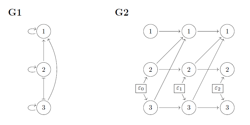
The submatrices of \(M\), \(M_{ij}\), and of \(D\), \(D_{ij}\), are \(2\times 2\)-matrices. We define a graph in terms of the matrices M and D. It has nodes \(1, \ldots, n\), it has a directed edge \(i\rightarrow j\) if \(M_{ji}\) may be nonzero, and it has a blunt edge if \((DD^T)_{ij}\), \(i\neq j\), may be nonzero. The graph encodes the sparsity patterns of the matrices, and we see that the sparsity of the above matrices is encoded by the graph G1. The simulated movement data in the gif was generated from a system with the above sparsity in matrices \(M\) and \(D\).
We say that this kind of graph is a directed correlation graph (cDG). The blunt edges represent symmetric dependence and the directed edges represent asymmetric dependence. ((We note that the blunt edges do not represent marginalization, but specifically correlation in the noise processes driving the model – for stochastic processes this is not the same as partial observation)). To aid our understanding of this kind of graph, we can construct an unrolled version (graph G2). In graph G1, each node (circle) represents an entire two-dimensional process, i.e., the movement of one animal. In graph G2, each node represents the location of an animal at a single point in time, that is, G2 represents a discretized version of the movement process. The \(\varepsilon\)-variables represent external stimulus creating dependence between noise processes.
A cDG is more useful than it may look at first glance! If we want to predict the immediate movement of Animal \(j\), say, in the herd, the cDG tells us that we only need to know the position of all animals with an arrow pointing into Animal \(j\). Moreover, the immediate movement correlates only with the immediate movements of all animals connected to Animal \(j\) via a blunt edge. Suppose now that there is no arrow from \(i\) to \(j\), but that we also do not observe the entire herd. Will Animal \(i\) then be predictive of the immediate movements of Animal \(j\) given the position of all other observed animals? We show a key result, known as the global Markov property, to help answer this question. From the cDG one can use a purely graphical algorithm (just computations using the graph) to check conditions that are sufficient for Animal \(i\) not to be predictive given the other observed animals. ((this graphical criterion is known as \(\delta\)- or \(\mu\)-separation and is an adaptation of \(d\)-separation)). In summary, we can learn, from the graph alone, probabilistic facts about which groups of animals can be ignored when predicting immediate movement of other animals. This is quite useful.
Having established a useful link between the evolution of the stochastic differential equation model above and its associated graph, the paper investigates the properties of the graphs. When we have two graphs on the same node set (i.e., only the edges differ), a natural question is whether they represent the same dependence structure. In the animal movement example, we may think of each possible graph on three nodes as encoding a certain set of movement (in)dependences. If we are to learn graphs from observation of animal movement, then we need to understand which graphs encode the same set of movement (in)dependences. The paper characterizes this kind of equivalence. Finally, the paper shows that determining Markov equivalence of two directed correlation graphs is computationally hard (it is coNP-complete).
This work was supported by VILLUM FONDEN (research grant 13358).