Minimax Estimation and Identity Testing of Markov Chains

The distribution setting

Estimation/Learning. A fundamental problem in statistics is to estimate a probability distribution from independent samples. Consider an alphabet \(\mathcal{X}\) of size \(d\), and draw \(X_1, X_2, \dots, X_n\) from a distribution \(\mu\) over \(\mathcal{X}\). How large must \(n\) –the sample size– be in order to obtain a good estimator \(\hat{\mu}(X_1, \dots, X_n)\) of \(\mu\)? In order to make the question precise, we choose a notion of distance \(\rho\) between distributions, pick two small numbers \(\delta, \varepsilon > 0\) and can for instance say that an estimator is good, when with high probability \(1 - \delta\) over the random choice of the sample, the estimator is \(\varepsilon\) close to the true distribution. Framed as a (probably approximately correct) minimax problem, we define the sample complexity of the problem to be \[\begin{equation*} n_0(\varepsilon, \delta) = {\mathrm{\arg\min}} \{n \in \mathbb{N} \colon \min_{\hat{\mu}} \max_{\mu} \mathbb{P}(\rho(\hat{\mu}(X_1, \dots, X_n), \mu) > \varepsilon) < \delta\}, \end{equation*}\] where the maximum is taken over all distributions over \(d\) bins, and the minimum over all estimators. The problem of determining \(n_0\) is then typically addressed by providing two distinct answers. On one hand, we construct an estimator that would be good for any distribution given that \(n > n_0^{UB}\). Conversely, we set up a hard problem such that no estimator can be good when \(n < n_0^{LB}\). This essentially leads to \[\begin{equation*} n_0^{LB} \leq n_0 \leq n_0^{UB}, \end{equation*}\] and the smaller the gap between the upper and lower bounds, the better we understand the sample complexity of the statistical problem. With respect to the total variation distance \[\begin{equation*} \rho_{TV}(\mu, \mu') = \frac{1}{2} \sum_{x \in \mathcal{X}} |\mu(x) - \mu'(x)|, \end{equation*}\] it is folklore (see e.g. Waggoner (2015)) that \[\begin{equation*} n_0(\varepsilon, \delta) \asymp \frac{d + \log 1 /\delta}{\varepsilon^2}, \end{equation*}\]and that the empirical distribution achieves the minimax rate ( \(f \asymp g\) stands for \(c g \leq f \leq C g\) for two universal constants \(c,C \in \mathbb{R}\)). The take-away is that if we want to estimate a distribution over \(d\) symbols w.r.t total variation, the statistical hardness of the problem grows roughly linearly with the support size.

Identity testing. A different problem is to imagine that the practitioner has access to independent data sampled from some unknown distribution \(\mu\) and the full description of a reference distribution \(\bar{\mu}\). They then have to make a determination as to whether the data was sampled from \(\bar{\mu}\), or from a distribution which is at least \(\varepsilon\) far from \(\mu\) (composite). To better compare with the previous problem, we keep the total variation metric. We briefly note that the unknown distribution being closer than \(\varepsilon\), but not equal to \(\bar{\mu}\), is not among the choices –we require separation of the hypotheses.

One can come up with a simple ``testing-by-learning” approach to solve the problem. First estimate the unknown distribution down to precision \(\varepsilon/2\) using the sample, and then verify whether the estimator is close to \(\hat{\mu}\). However, identity testing corresponds to a binary, seemingly easier question. As such, we would expect the sample complexity to be less than that of the estimation problem. Among the first to investigate the problem in the case where \(\bar{\mu}\) is the uniform distribution was Paninski (2008), who showed that the complexity of the problem grows roughly as the square root of the alphabet size, i.e. much more economical than estimation. For this uniformity testing problem, several procedures are known to achieve the minimax rate (although not all work in all regimes of parameters). One can for instance count the number of collisions in the sample, count the number of bins appearing exactly once in the sample, or even compute a chi-square statistic. In fact, the complexity for the worst-case \(\bar{\mu}\) has been pinned-down to (see Diakonikolas et al. (2017)) \[\begin{equation*} n_0(\varepsilon, \delta) \asymp \frac{\sqrt{d \log 1 /\delta} + \log 1 /\delta}{\varepsilon^2} \end{equation*}\] In recent years, the sub-field of distribution testing has expanded beyond this basic question to investigate a vast collection of properties of distributions –see the excellent survey of Canonne (2020) for an overview.

The Markovian setting

We depart from independence and increase the richness of the process by considering the Markovian setting. More specifically, we wish to perform statistical inference from sampling a ``single trajectory” of a Markov chain, i.e. a sequence of observations \(X_1, X_2, \dots, X_m\) where \(X_1\) is drawn from an unknown, arbitrary initial distribution, and the transition probabilities governing \(X_t \to X_{t+1}\) are collected in a row-stochastic matrix \(P\). It is a challenging but fair representation of a process outside of the control of the scientist, that cannot for example be restarted, or set to any particular state. For simplicity of the exposition below, we will assume that \(P\) is ergodic and time reversible, but the approach and results can be extended to the periodic or non-reversible cases (see the concluding remarks). To measure distance between Markov chains, we here consider the infinity matrix norm between their respective transition matrices, \[\begin{equation*} \rho(P, P') = \|P - P'\|_{\infty} = \max_{x \in \mathcal{X}} \sum_{x' \in \mathcal{X}} |P(x,x') - P'(x,x')|, \end{equation*}\] and recognize that it corresponds to a uniform control over the conditional distributions defined by each state w.r.t total variation. The notion of sample size (we have only one sample) is replaced with the trajectory length. Definitions of the minimax estimation and identity testing problems follow from this sampling model and choice of metric. Since the number of parameters in the model jumps approximately from \(d\) to \(d^2\), a first guess would be to replace \(d\) by \(d^2\) in the sample complexities obtained in the iid setting. However, our ability to test or estimate the conditional distribution defined by a state is restricted by the number of times we visit it. For instance, if the stationary probability –the long run probability of visit– of some states is small, or if the chain exhibits a sticky behavior, we would not be able to make decisions unless the trajectory length increases accordingly.

Estimation/Learning. Finite sample analyses for the problem are relatively recent, with the first treatments of Hao, Orlitsky, and Pichapati (2018) in expectation and Wolfer and Kontorovich (2019) in the PAC framework.

We estimate the unknown \(P\) with the empirical tally matrix, where \(\widehat{P}(x,x')\) is computed by counting transitions from \(x\) to \(x'\) and dividing by the number of visits to \(x\) (modulo some mild smoothing). Tighter upper and lower bounds on the sample complexity were later obtained (see Wolfer and Kontorovich (2021)) \[\begin{equation*} \begin{split} c \left( \frac{d}{\pi_{\star} \varepsilon^2} + \frac{d \log d}{{\gamma_\star}} \right) \leq m_0(\varepsilon, \delta) \leq C \left( \frac{d + \log 1/(\varepsilon \delta)}{\pi_{\star} \varepsilon^2} + \frac{\log 1/(\pi_\star \delta)}{\pi_{\star} {\gamma_\star}} \right) \quad \\ \end{split} \end{equation*}\] where \(c, C > 0\) are universal constants, \(\pi_\star = \min_{x \in \mathcal{X}} \pi(x)\) with \(\pi\) the stationary distribution of \(P\), and \(\gamma_\star\) is the absolute spectral gap –the difference between the two largest eigenvalues of \(P\) in magnitude– that largely controls the mixing time of the (reversible) Markov chain. The bounds are independent of the starting state, but require a priori knowledge of bounds on \(\pi_\star\) and \(\gamma_\star\) to be informative. Notably, procedures exist to efficiently estimate \(\pi_\star\) and \(\gamma_\star\) from the data Hsu et al. (2019) and Wolfer (2022).

We witness a stark difference between the iid and Markovian settings: a phase transition appears in the sample complexity. Roughly speaking and taking \(\varepsilon\) as a constant, when the mixing time of the chain is larger than the number of states, the second term becomes the dominant one, i.e. the difficulty of estimation is chiefly controlled by how well we can navigate among the states. When the chain mixes more quickly, moving from state to state is not bottleneck, and the harder task is the estimation of the respective conditional distributions. An additional caveat is that the chain will generally not visit all states equally in the long run. As a result, the sample complexity necessarily depends on the proportion \(\pi_\star\) of the trajectory spent in the least visited state. The astute reader may notice that when the mixing time is small and the stationary distribution is uniform (\(P\) is doubly stochastic), we recover up to logarithmic factors the previously intuited complexity of \(d^2/\varepsilon^2\).

Identity testing. For the Markov chain identity testing problem (still w.r.t the matrix uniform norm), we rely on a two-stage testing procedure. First, we verify that we visited all states about \(\sqrt{d}/\varepsilon^2\) times. As a second step, we perform identity testing of all conditional distributions. The Markov property ensures that our transition observations are drawn independently from the conditional distribution, thus that we can rely on one of the known iid testing procedures as a black-box. We obtain the below-listed upper and lower bounds on the sample complexity (see Wolfer and Kontorovich (2020)) \[\begin{equation*} \begin{split} c \left( \frac{\sqrt{d}}{\bar{\pi}_\star \varepsilon^2} + \frac{d}{\bar{\gamma}_\star} \right) \leq m_0(\varepsilon, \delta) \leq C \left( \frac{\sqrt{d}}{\bar{\pi}_\star \varepsilon^2} \log \frac{d}{\varepsilon \delta} + \frac{\log 1/(\bar{\pi}_\star \delta)}{\bar{\pi}_\star \bar{\gamma}_\star} \right) \qquad \\ \end{split} \end{equation*}\]

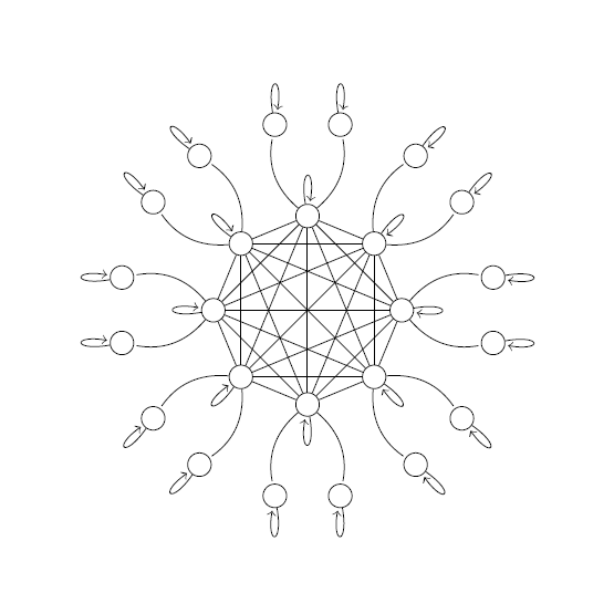
Figure 1: Topology of class of Markov chains achieving the lower bounds in \(d /\gamma_\star\).

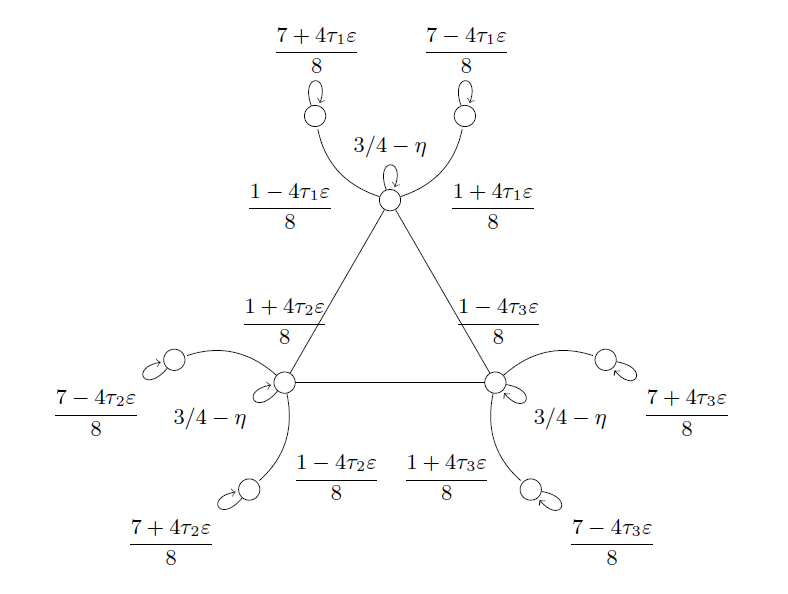
Figure 2: Example of the class in Figure 1 with \(d = 9\), \(\tau \in \{-1, 1\}^3\) and \(0 < \eta \ll 1\). The mixing time of the chain is of the order of \(1/\eta\), and is decoupled from the proximity parameter \(\varepsilon\).

Perhaps surprisingly, the bounds only depends on properties \(\bar{\pi}_\star\), \(\bar{\gamma}_\star\) of the reference stochastic matrix. As a matter of fact, the unknown chain need not even be irreducible for the procedure to work. A quadratic speed-up also appears in the bounds, which will affect the dominant term when the chain mixes faster than \(\sqrt{d}\).

It is instructive to inspect the set of reversible Markov chains that achieves the lower bounds in \(d / \gamma_\star\) (see Figure 1 and Figure 2). Every element consists of an “inner clique” and an “outer rim”. The inner clique can be made arbitrarily sticky in the sense that the chain will only move from one state to another within the clique with underwhelming probability \(\eta\), which has an overall slowing effect on the mixing time of the chain. On the other hand, being on one state of the clique, the chain has at least constant –but parametrizable– probability of reaching one of the two connected states in the outer rim. In order to distinguish between two chains where one of the inner nodes has \(\varepsilon\)-different transition probabilities towards the rim than the other, the trajectory will necessarily have to go through a large fraction of the states.

Related work and closing comments. As mentioned earlier in this note, the results are valid for a substantially larger class of chains. In the non-reversible setting, the absolute spectral gap can readily be replaced with the pseudo-spectral gap Paulin (2015), and if the chain is irreducible (but possibly periodic), one can instead perform inference on the lazy process governed by \((P+I)/2\), which can be simulated with an additional fair coin. More recently, Chan, Ding, and Li (2021) investigated the Markov chain minimax learning and testing problems by considering cover times instead of mixing times.

We end this post by stressing that the minimax rates pertain to the choice of metric. We refer the interested reader to Daskalakis, Dikkala, and Gravin (2018), Cherapanamjeri and Bartlett (2019) and Fried and Wolfer (2022), who analyze the identity testing problem with respect to a different notion of discrepancy between Markov chains. Although the last-mentioned framework can so far only handle reversible chains, it advantageously leads to minimax rates that are independent of mixing or hitting.