Introduction
Migration is a multifaceted phenomenon including macro-, meso-, and micro-triggers that, when combined, decide an individual’s final decision to migrate. Apart from being an essential component of population change, migration is also an important component of population estimates and labor market force estimations. Jennissen (2004) argues that the presence of migrant populations has a favorable impact on natural population growth since migrants’ age characteristics and fertility rates are often greater than those of the indigenous population. Furthermore, the migration problem is far more significant for population growth in European nations, which are generally seeing a drop in natural population increase. In this environment, it’s critical to identify and quantify the factors involved in the decision to migrate. Income disparities or income inequality, economic development, the tax system, the economic cycle, the availability of new job opportunities, unemployment, and other variables have been highlighted as factors affecting migration by several migration theories (Kumpikaite and Zickute, 2012). People migrate for a variety of reasons, including improved living conditions or an escape from adverse circumstances in their native country. This is the foundation of Lee’s (1966) push and pull hypothesis, which is one of the primary neo-classical migration hypotheses. Individuals are influenced by supply-push forces to leave their home country, while demand-pull variables draw migrants to the destination country.
Panel data analysis is the study of datasets in which entities are observed through time and allows for the management of missing variables without having to examine them. By examining changes in the dependent variable across time, one may rule out the impact of neglected factors that fluctuate between entities but remain constant over time. The basic premise is that if unobserved factors (such as those peculiar to nations) influence the dependent variable yet stay constant over time, the changes in the dependent variable must come from other sources.
The notation for panel data will be the following: \[\begin{equation} (x_{1,it}, x_{2,it}, ..., x_{k,it}, y_{it}), i=1,2, ..., n; t=1,2, ..., T \end{equation}\]
where i is the subscript for the entity being observed (in our case study the country) and t is the subscript for the date at which the entity is observed (in our case study the year). Using these notations we would have data for the variables \[\begin{equation} x_1, x_2, ..., x_k, y \end{equation}\]
The fixed effects approach
The fixed effects model would be written as:
\[\begin{equation} y_{it}=\beta_1 x_{1,it} + \beta_2 x_{2,it} + \dots + \beta_k x_{k,it} + \alpha_i + u_{it} \end{equation}\]where:
- \(x_{j,it}\) represents the value of regressor j, for entity i and time period t.
- \(\beta_j\) represents the coefficients of the independent variables, that do not vary across individuals.
- \(\alpha_i\) represents the entity specific intercepts.
The random effects approach
the unobserved variable specific to the individual entity is encompassed in the error term. The entities will have a common mean value for the intercept (let’s denote this with \(\alpha\)) and the specific differences in the intercept values of each country would be reflected in an error term (denoted with \(\epsilon_i\)).
\[\begin{equation} y_{it}=\alpha + \sum_{j=1}^{k} \beta_j x_{j,it} + \epsilon_i + u_{it} \end{equation}\]We will obtain a composite error term, which is composed of \(\epsilon_i\), the individual (cross section) specific error \(u_{it}\) and a combined cross section and time series error: \[\begin{equation} w_{it}=\epsilon_i + u_{it} \end{equation}\]
Thus substituting both equations we obtain: \[\begin{equation} y_{it}=\alpha + \sum_{j=1}^{k} \beta_j x_{j,it} + w_{it} \end{equation}\]
The main benefit of using panel data related techniques is that individual heterogeneity of individual entities (countries) can be explicitly taken into account in panel data estimation; additionally, panel data offers “more informative data, more variability, less collinearity, more degrees of freedom, and more efficiency” by combining time series and cross-sectional observations (Baltagi, 2001).
The database involved
The Crude Rate of Net Migration plus adjustment is the dependent variable in both estimated models. It is calculated as the annual ratio of net migration to the average population. It is expressed in terms of 1000 people (of the average population). The difference between the total number of immigrants and the total number of emigrants is referred to as net migration; statistical adjustments refers to adjusting net migration by taking the difference between total population change and natural change; the indicator roughly covers the difference between inward and outward migration. In the model, the variable is called “Net Migration.”
The independent variables in the models are as follows:
- Unemployment: The long-term unemployment rate is the percentage of people who have been jobless for more than a year out of the total number of people who are working.
- Earnings (adjusted): The adjusted gross disposable income of households divided by the PPP (purchasing power parities) of the actual individual consumption of households and by the entire resident population (in purchasing power standard (PPS) per inhabitant) yields gross disposable income of households per capita.
- Gini Coefficient (of equivalised disposable income): A relationship between the cumulative shares of the population disposed based on equivalised disposable income and the cumulative share of the equivalised total disposable income received by the population is defined as the Gini Coefficient (of equivalised disposable income).
- Poverty: The at-risk-of-poverty rate is the proportion of people whose equivalised disposable income is less than the risk-of-poverty threshold, which is set at 60% of the national median equivalised disposable income.
- Economic Freedom: A 0–10 scale that assesses the degree of economic liberty in five key areas: government size, legal system, sound money, international trade freedom, and regulation.
- Hospital beds: the number of beds available in hospitals; the variable is calculated per 100,000 people.
- Health spending: the overall amount spent on health as a proportion of GDP ( percent ).
Eurostat is the data source for all variables except Economic Freedom. The Fraser Institute is the source of data for the Economic Freedom Index. Data was collected for 25 EU nations over a period of 18 years, from 2000 to 2017.
Figure 1 depicts the dispersion of average Net Migration rates for EU nations for the period 2000–2017. Lithuania (-8.84), Latvia (-7.19), and Romania (-7.19) are the nations with the lowest average Net Migration between 2000 and 2017. (-5.48). Bulgaria, Estonia, Poland, and Slovakia all had negative Net Migration averages over the time period studied. This was to be expected, given that these economies in Central and Eastern Europe are generally migration-sending countries (Jennissen, 2004). Luxembourg, Spain, and Sweden, on the other hand, have the greatest average Net Migration rates, indicating that they are typically migrant-receiving nations. The Net Migration Rate’s behavior proposes that the group of nations be divided into two: typically sending and traditionally receiving countries.
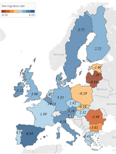
Figure 1 – Average Net Migration for the period 2000 – 2017 for the EU countries; source: author’s processing in Tableau, based on Eurostat data.
Figure 2 depicts the significant relationship between real GDP/capita, chain linked volume (2010) in Euro/capita, and net migration rate (averages from 2000 to 2017 were used). Nations with lower GDP per capita also have negative or low Net Migration rates, indicating that “poorer” countries are more likely to be the source of migrant flows (sending countries). Nations with greater GDP/capita, on the other hand, have higher migration rates, implying that they are primarily receiving countries for migrants.
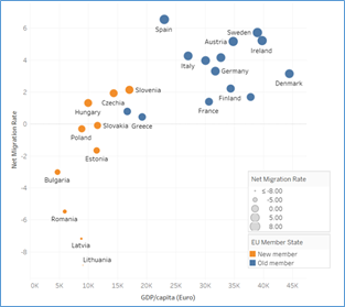
Figure 2 – Net Migration rate vs. GDP/capita – comparison between old and new EU member states; source: author’s processing in Tableau, based on Eurostat data.
The tendency of Net Migration for old and new member states warrants the dataset being separated into two categories. It is clear from this research that the group of New Member States acts as Migrant Sending Countries for the whole time under consideration, while the Old Member States operate as Migrant Receiving Countries. As a result, the empirical application will be split into two parts: one model for the Old member nations and then another model (Table 1) for the New member states (Table 2).
Table 1. Results of estimation for fixed and random effects models for Old Member States; source: author’s own results
| Fixed Effects | Random Effects | |
|---|---|---|
| Unemployment | -1.0468*** (0.0903) | -1.0295*** (0.0881) |
| Ln_Income | 4.9042** (2.4037) | 8.1458*** (1.5631) |
| Gini | -0.1777 (0.1691) | -0.3282** (0.1391) |
| Poverty | 0.6876*** (0.1657) | 0.7331*** (0.1417) |
| Economic Freedom | -4.5181*** (1.5230) | -2.9796*** (1.0923) |
| Health Expenditure | -1.4840*** (0.4175) | -1.7844*** (0.2965) |
| Intercept | -1.6247 (25.7912) | -40.0461** (17.8813) |
| R2 | Within 0.4184 Between 0.6589 Overall 0.5056 | Within 0.4109 Between 0.8405 Overall 0.5828 |
| F | 29.85*** | 229.47*** (Wald chi2) |
| Corr (u_i, xb) | 0.2190 | 0 (assumed) |
| Sigma_u | 2.0795 | 1.3274 |
| Sigma_e | 3.0081 | 3.0081 |
| Rho | 0.3233 | 0.1629 |
*** Significant at 0.01; ** Significant at 0.05
(standard errors of the coefficients are reported in parenthesis)
Table 2. Results of estimation for fixed and random effects models for New Member States; source: author’s own results
| Fixed Effects | Random Effects | |
|---|---|---|
| Unemployment | -0.3900** (0.1547) | -0.3893*** (0.1461) |
| Gini | -0.3527** (0.1377) | -0.5432*** (0.1226) |
| Economic Freedom | 4.3493*** (1.1280) | 4.3283*** (1.0755) |
| Health Expenditure | -1.1240* (0.5841) | -0.4513 (0.4765) |
| Intercept | -15.6762 (8.0909) | -13.3742** (7.5791) |
| R2 | Within 0.1663 Between 0.0205 Overall 0.0855 | Within 0.1483 Between 0.5198 Overall 0.3147 |
| F | 8.28*** | 38.90*** (Wald chi2) |
| Corr (u_i, xb) | -0.1069 | 0 (assumed) |
| Sigma_u | 3.9181 | 2.2254 |
| Sigma_e | 3.5999 | 3.5999 |
| Rho | 0.5422 | 0.2765 |
*** Significant at 0.01; ** Significant at 0.05; * Significant at 0.1
(standard errors of the coefficients are reported in parenthesis)
The influence of macroeconomic factors on the Crude Rate Net Migration of European economies was quantified using panel data regression models. A preliminary study of the dependent variable’s distribution reveals that the net migration rate differs across Old Member States (migrant-receiving nations) and New Member States (sending countries for migrants). As a result, we opt to estimate two models for the two sets of nations, following Mihi-Ramirez et al. (2017) method’s. Unemployment rate, per capita income, Gini coefficient, poverty rate, Economic Freedom Index, and two other characteristics relating to the health system were included as independent variables (number of beds in hospitals and health expenditure as percentage in GDP). The analysed period was 2000 – 2017.
The findings corroborated migratory economic theory. In terms of the labor market, unemployment is a large and powerful supply push factor for migration. Only for the Old Member states does income appear as a key influence, validating the neo-classical economic theory of migration, which claims that variations in earnings across nations are one of the main factors driving labor movement (Massey et al, 1993). Moving on to the social component, the Gini coefficient has been established as a strong driving force behind migration in both Old and New Member States. Poverty appears to be a factor with reduced explanatory power, with a positive coefficient for the Old member states and no significance for the New member states.
In terms of Economic Freedom, the factor has a considerable beneficial impact on net migration rates only in the New Member States.
Furthermore, health-related macroeconomic factors were included in the model, as well as the circular cumulative causation hypothesis, which states that variations in standard of living across nations are the primary cause of migration (Massey et al. 1993). The health system, on the other hand, could not be proven to be a factor of migration.
Because international migration has such a substantial impact on European population dynamics, understanding and analyzing the factors that influence international migration is critical. The findings of this study might be utilized not just to produce migration forecasts, but also to establish migration policies that would improve migrants’ labor and social integration.
Author:
Smaranda Cimpoeru, PhD
Department of Statistics and Econometrics, The Bucharest University of Economic Studies
E-mail: smaranda.cimpoeru@csie.ase.ro