Overview
Bayesian nonparametric (BNP) models are a prominent tool for performing flexible inference with a natural quantification of uncertainty. Traditionallly, flexible inference within a homogeneous sample is performed with exchangeable models of the type \(X_1,\dots, X_n|\tilde \mu \sim T(\tilde \mu)\), where \(\tilde \mu\) is a random measure and \(T\) is a suitable transformation. Notable examples for \(T\) include normalization for random probabilities (Regazzini et al., 2003), kernel mixtures for densities (Lo, 1984) and for hazards (Dykstra and Laud, 1981; James, 2005), exponential transformations for survival functions (Doksum, 1974) and cumulative transformations for cumulative hazards (Hjort, 1990).
Very often, though, the data presents some structural heterogeneity one should carefully take into account, especially when analyzing data from different sources that are related in some way. For instance this happens in the study of clinical trials of a COVID-19 vaccine in different countries or when understanding the effects of a certain policy adopted by multiple regions. In these cases, besides modeling heterogeneity, one further aims at introducing some probabilistic mechanism that allows for borrowing information across different studies. To achieve this goal, in the last 20 years a wealth of BNP models that rely on partial exchangeability have been proposed (see Cifarelli & Regazzini (1978) for prioneering ideas, MacEachern (1999, 2000) for seminal results and Quintana et al. (2021) for a recent review). The general recipe consists in assigning a different random measure \(\tilde \mu_i\) to every data source or group of observations and then introduce flexible forms of dependence between the random measures. For simplicity we stick to the case of two groups, so that the partially exchangeable models are of the general form \[\begin{equation} \tag{1} X_1,\dots,X_{n_1}| (\tilde \mu_1, \tilde \mu_2) \stackrel{\text{iid}}{\sim} T(\tilde \mu_1); \qquad \qquad Y_1, \dots, Y_{n_2} | (\tilde \mu_1, \tilde \mu_2) \stackrel{\text{iid}}{\sim} T(\tilde \mu_2); \end{equation}\] and \((\tilde \mu_1, \tilde \mu_2) \sim Q\) is a vector of dependent random measures. The borrowing of information across different groups is regulated by the amount of dependence between random measures. One can picture two extreme situations:
- When the random measures are completely dependent, that is, \(\tilde \mu_1 = \tilde \mu_2\) almost surely, the observations are fully exchangeable and there is no distinction between the different groups. In such case we denote the random measures as \((\tilde \mu_1^\text{ex}, \tilde \mu_2^\text{ex})\).
- When the random measures are independent, the two groups of (exchangeable) observations are independent and thus do not interact.
Thus, it is crucial to translate one’s prior beliefs on the dependence structure into the specification of the model. Interestingly, though there have been many proposals on how to model dependence, few results on how to measure it are available. The current state-of-the-art is given by the pairwise linear correlation between \(T(\tilde \mu_1)\) and \(T(\tilde \mu_2)\), which provides a useful proxy based on the first two moments of the random measures, but it does not take into account their whole infinite-dimensional structure. We thus look for a measure of dependence with the following properties:
- It is model non-specific (i.e., it does not depend on the choice of transformation \(T\));
- It is based on the whole infinite-dimensional distribution of BNP priors;
- It can be naturally extended to more than 2 groups of observations;
- It can be strictly bounded in terms of the hyperparameters of BNP models.
We point out that this last property is fundamental because it allows to fix the hyperparameters of BNP models so to achieve the desired level of dependence.
Proposal
Our proposal is based on two main ideas:
In partially exchangeable models (1) all the dependence between different groups of observations is introduced at the level of the random measures. Thus, we can measure the dependence directly in terms of the underlying vector of random measures \((\tilde \mu_1, \tilde \mu_2)\). This ensures Property 1.
Complete dependence (\(\tilde \mu_1^{\text{ex}} = \mu_2^{\text{ex}}\) almost surely) coincides with the full exchangeability of the observations, which can thus be pictured as a degenerate distribution in the space of joint distributions \(\{ \mathcal{L}(\tilde \mu_1, \tilde \mu_2) | \mathcal{L}(\tilde \mu_1) = \mathcal{L}(\tilde \mu_2) \}\), where \(\mathcal{L}\) denotes the probability law of a random object (Figure 1). A natural way to measure dependence of any other joint distribution \((\tilde \mu_1, \tilde \mu_2)\) is then to measure the distance from the extreme case \((\tilde \mu_1^{\text{ex}}, \tilde \mu_2^{\text{ex}})\). This ensures Property 2 and Property 3. Informally, we refer to the distance from exchangeability, with the underlying idea that the observations in (1) are partially exchangeable and, under complete dependence of the random measures, one retrieves full exchangeability of the observations.
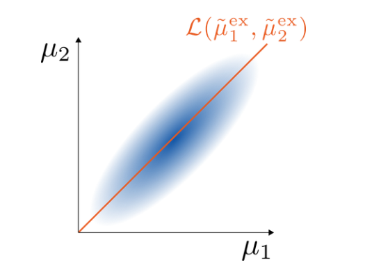
The choice of the distance on the laws of vectors of random measures is very delicate. On one hand we look for an intuitive notion of distance with a natural geometrical interpretation, on the other hand we also want to show Property 4, and these are clearly two competing aspects. We define \[\begin{equation} \tag{2} d_{\mathcal{W}}\bigg( \mathcal{L}\begin{pmatrix} \tilde \mu_1 \\ \tilde \mu_2 \end{pmatrix}, \mathcal{L} \begin{pmatrix} \tilde \mu_1^{\text{ex}} \\ \tilde \mu_2^{\text{ex}} \end{pmatrix} \bigg) = \sup_A W\bigg( \mathcal{L}\begin{pmatrix} \tilde \mu_1(A) \\ \tilde \mu_2(A) \end{pmatrix}, \mathcal{L} \begin{pmatrix} \tilde \mu_1^{\text{ex}}(A) \\ \tilde \mu_2^{\text{ex}} (A)\end{pmatrix} \bigg), \end{equation}\] where \(W\) is the Wasserstein distance (of order 2) between probability distributions in \(\mathbb{R}^2\). We briefly recall that if \(C(P,Q)\) = \(\{(X,Y): \mathcal{L}(X) = P; \mathcal{L}(Y) = Q\}\) denotes the set of couplings between two probabilities \(P\) and \(Q\), then \[\begin{equation} \tag{3} W(P,Q)^2 = \inf_{(X,Y) \in C(P,Q)} \mathbb{E} \|X-Y\|^2. \end{equation}\] Because of its strong geometric properties, the Wasserstein distance is ideal to compare distributions with different support as in our case (see Figure 1). Indeed, other common distances or divergences would not provide an informative notion of discrepancy in this context (e.g. total variation distance, Hellinger distance, KL-divergence). As it is often the case, there is a trade-off between the naturalness of a distance and our ability to find closed forms expressions. In particular, we have to deal with the following challenges:
In general one can prove that the infimum in (3) is a minimum, that is, that there exists an optimal coupling. Nonetheless, since we are dealing with probabilities in \(\mathbb{R}^d\) for \(d>1\), a general expression for the optimal coupling is not available with very few exceptions (e.g., between multivariate normal distributions).
Even if one finds the optimal coupling, the expression of the Wasserstein distance amounts to evaluating a (difficult) multivariate integral.
Many noteworthy models in the BNP literature are based on dependent random measures with jointly independent vectors which, in analogy with the 1-dimensional case, we call completely random vectors. The law of such vectors is specified in an indirect way through a multivariate Lévy measure. Thus, we need to develop strict bounds in terms of the Lévy measures to find closed form expressions that depend on the hyperparameters of the models (Property 4).
Results
In our work (Catalano et al., 2021) we face the challenges above and obtain the following results:
When dealing with completely random vectors, \((\tilde \mu_1(A), \tilde \mu_2(A))\) can always be approximated with compound Poisson (CP) distributions. We find upper bounds of the Wasserstein distance between completely random vectors in terms of the Wasserstein distance between the jumps of the corresponding CP approximations, whose law is expressed directly in terms of the Lévy measures.
We find a general expression for the optimal coupling between the jumps of the CP approximation of \((\tilde \mu_1, \tilde \mu_2)\) and the ones of the CP approximation of \((\tilde \mu_1^\text{ex}, \tilde \mu_2^{\text{ex}})\).
Once we have found the optimal coupling, the Wasserstein distance between the jumps of the CP approximations amounts to the evaluation of a multivariate integral. We develop case-by-case analyses to evaluate these multivariate integrals numerically.
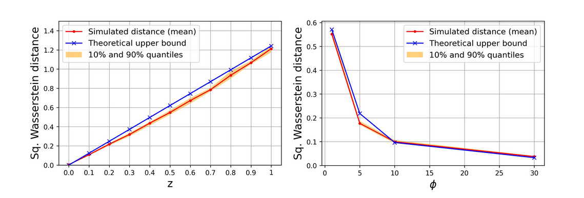
Putting these three elements together, we are able to derive strict upper bounds of the distance in (2) for noteworthy models in the BNP literature, which include compound random measures (Griffin & Leisen, 2017; Riva-Palacio & Leisen, 2019), Clayton Lévy copula (Tankov, 2003; Epifani & Lijoi, 2010) and additive models (Griffiths & Milne, 1978; Lijoi et al., 2014). These upper bounds are expressed in terms of the hyperparameters of the corresponding models (see Figure 2) and thus enable a principled prior specification of their dependence structure.
Discussion and further work
We highlight two take-home messages:
We can use the Wasserstein distance to build a natural and tractable distance on a wide class of (vectors of) random measures. This opens the way to many possible uses of a distance between infinite dimensional random structures, going beyond the measurement of dependence.
A natural way to measure the dependence between infinite-dimensional random quantities is to evaluate the distance from an extreme situation, as the one of complete dependence.
In Catalano et al (2021) we have moved the first steps. Yet, there are a number of questions that still remain open. In particular,
We measure dependence in terms of distance from the extreme situation of complete dependence. How can we simultaneously quantify the discrepancy from the other extreme, that is, independence?
Using the distance from exchangeability to measure dependence is useful for relative comparisons between dependence structures (“\(\tilde \mu_1\) is more dependent than \(\tilde \mu_2\)”) but prevents absolute quantifications of dependence (“\(\tilde \mu\) has an intermediate dependence structure”). In order to extend the measure in this direction we need to find the maximum possible value of the distance from exchangeability.
In Catalano et al (2022+) we deal with these questions. Their answer sheds light into the deep geometric properties of the Wasserstein distance, which are key to the definition of a Wasserstein Index of Dependence in [0,1]: our goal since the beginning. This opens interesting research directions on how to use the index to assess heterogeneity in the data, going beyond the restrictive assumption of independence.
References
Catalano, M., Lavenant, H., Lijoi, A., Prünster, I. (2022+). A Wasserstein Index of Dependence for Random Measures. arXiv:2109.06646.
Catalano, M., A. Lijoi, and I. Prünster (2021). Measuring dependence in the Wasserstein distance for Bayesian nonparametric models. Ann. Statist. 49(5), 2916–2947.
Cifarelli, D.M. & Regazzini, E. (1978). Nonparametric statistical problems under partial exchangeability: The role of associative means. Technical Report.
Doksum, K. (1974). Tailfree and neutral random probabilities and their posterior distributions. The Annals of Probability, 2(2):183–201.
Dykstra, R. L. and Laud, P. (1981). A Bayesian nonparametric approach to reliability. The Annals of Statistics, 9(2):356– 367.
Epifani, I. and Lijoi, A. (2010). Nonparametric priors for vectors of survival functions. Statist. Sinica 20 1455–1484.
Hjort, N. L. (1990). Nonparametric Bayes estimators based on beta processes in models for life history data. The Annals of Statistics, 18(3):1259–1294.
Griffin, J. E. & Leisen, F. (2017). Compound random measures and their use in bayesian non-parametrics. J. Royal Stat. Soc. Ser. B 79, 525–545.
Griffiths, R. C. and Milne, R. K. (1978). A class of bivariate Poisson processes. J. Multivariate Anal. 8 380–395.
James, L. F. (2005). Bayesian Poisson process partition calculus with an application to Bayesian Lévy moving averages. The Annals of Statistics, 33(4):1771–1799.
Lijoi,A., Nipoti,B. and Prünster, I. (2014). Bayesian inference with dependent normalized completely random measures. Bernoulli 20 1260–1291.
MacEachern, S. N. (1999). Dependent nonparametric processes. in ASA Proceedings of the Section on Bayesian Statistical Science, Alexandria, VA: American Statistical Association.
MacEachern, S. N. (2000). Dependent Dirichlet processes. Tech. Report, Ohio State University.
Riva Palacio, A. and Leisen, F. (2021). Compound vectors of subordinators and their associated positive Lévy copulas. J. Multivariate Anal. 183.
Quintana, F. A., Müller, P., Jara, A., and MacEachern, S. N. (2021). The dependent Dirichlet process and related models. Statistical Science, to appear.
Tankov, P. (2003). Dependence structure of spectrally positive multidimensional Lévy processes. Unpub- lished Manuscript.