This is an updated version of a blog post on RIKEN AIP Approximate Bayesian Inference team webpage: https://team-approx-bayes.github.io/blog/mmd/
INTRODUCTION
A very old and yet very exciting problem in statistics is the definition of a universal estimator \(\hat{\theta}\). An estimation procedure that would work all the time. Close your eyes, push the button, it works, for any model, in any context.
Formally speaking, we want that for some metric \(d\) on probability distributions, for any statistical model \((P_\theta,\theta\in\Theta)\), given \(X_1,\dots,X_n\) drawn i.i.d from some \(P^0\) not necessarily in the model,
\[ d\left(P_{\hat{\theta}},P^0 \right) \leq \inf_{\theta\in\Theta} d\left(P_{\theta},P^0 \right) + r_n(\Theta), \]
where \(r_n(\Theta) \rightarrow 0\) when \(n\rightarrow \infty\) holds, either in expectation or with large probability.
Why would this be nice? Well, first, if the model is well specified, that is, \(P^0 = P_{\theta^0}\) for some \(\theta^0\in\Theta\), we would have:
\[ d\left(P_{\hat{\theta}},P^0 \right) \leq r_n(\Theta) \rightarrow 0, \]
so the estimator is consistent. But the ill-specified case is also relevant. Remember that “all models are wrong, some models are useful”. A very interesting case is Huber’s contamination model: assume that the data is drawn from the model, but might be corrupted with small probability. That is, \(P^0 = (1-\varepsilon) P_{\theta^0} + \varepsilon Q\) where \(\varepsilon\in[0,1]\) is small and \(Q\), the contamination distribution, can be absolutely whatever. Then we would have:
\[ d\left(P_{\hat{\theta}},P^0 \right) \leq d(P_{\theta^0},P^0) + r_n(\Theta) = d(P_{\theta^0},(1-\varepsilon) P_{\theta^0} + \varepsilon Q) + r_n(\Theta). \]
If the metric \(d\) is such that \(d(P_{\theta^0},(1-\varepsilon) P_{\theta^0} + \varepsilon Q) \leq C \varepsilon\) for some constant \(C\), we end up with
\[ d\left(P_{\hat{\theta}},P^0 \right) \leq C \varepsilon + r_n(\Theta), \]
which means that, as long as \(\varepsilon\) remains quite small, the estimator is still not too bad. That is, the estimator is robust to contamination.
THE MLE DOES NOT WORK
In case you believe that popular estimators such as Maximum Likelihood Estimator (MLE) is universal, surprise: it’s not.
First, if the model does not satisfy regularity assumptions, the MLE is not even defined. For example, consider a location model, that is, \(P_\theta\) has the density \[ p_\theta(x) = g(x-\theta) \] and consider \[ g(x) = \frac{\exp(-|x|)}{2\sqrt{\pi|x|}} . \] Obviously, the likelihood is infinite at each data point, that is, as soon as \(\theta\in\{X_1,\dots,X_n\}\), we have \[ \prod_{i=1}^n p_\theta(X_i) = +\infty. \] Even when the MLE is well defined, there are examples where it is known to be inconsistent [8]. It is also well known to be non robust to contamination in the data.
SOME EXAMPLES OF UNIVERSAL ESTIMATORS
The first example of universal estimator we are aware of: Yatracos’ estimator [7], with \(d\) being the total variation distance. It works with the rate \(r_n(\Theta) = [\mathrm{dim}(\Theta)/n]^{\frac{1}{2}}\) when \(\Theta\) is in some finite dimensional space. And it doesn’t work for nonparametric estimation. Still, it’s nice, and the paper is beautiful (and short). Equally beautiful is the book by Devroye and Lugosi [9] which studies many estimations methods for the total variation distance, including variants of Yatracos’ estimator.
Another example is Birgé, Barraud and Sart’s \(\rho\)-estimator [8], which satisfies a similar result for the Hellinger distance. If you want to read the paper, be aware: this is extremely difficult to prove! It is also very nice, because the Hellinger distance looks locally very similar to the KL in many models. In some sense, the \(\rho\)-estimator actually does what the MLE should do.
By the way. We live in the big data era, high dimensional data, big networks, more layers, you know. So it must be said that Yatracos’ estimator, and the \(\rho\)-estimators, cannot be used in practice. They require an exhaustive search in a fine discretization of the parameter space, don’t expect to do that with a deep NN. Don’t expect to do it either for a very shallow NN, not even for a linear regression in dimension 50 (as discussed later, a variant of Yatracos’ estimator by Devroye and Lugosi might be feasible, though).
MMD-ESTIMATION
Let us now describe yet another metric, and another estimator. This metric is based on kernels. So, let \(K\) be a kernel on the observations space, \(\mathcal{X}\). This means that there is an Hilbert space \(\mathcal{H}\), equipped with a norm \(\left\lVert\cdot\right\rVert _{\mathcal{H}}\), and a continuous map \(\Phi:\mathcal{X}\rightarrow \mathcal{H}\) such that \(K(x,x') = \left<\Phi(x),\Phi(x')\right>\).
Given a probability distribution \(P\) on \(\mathcal{X}\), let us define the kernel mean embedding
\[ \mu(P) = \int \Phi(x) P(\mathrm{d} x) = \mathbb{E} _{X \sim P }[\Phi(X)]. \]
Wait. Of course, this is not always defined! It is, say, if \(\int \left\lVert\Phi(x)\right\rVert_{\mathcal{H}} P(\mathrm{d} x) <+\infty\).
Now, it appears that some kernels \(k\) are known such that:
\(k(x,x) = \left\| \Phi(x) \right\|_{\mathcal{H}}^2 \leq 1\) for any \(x\), which in turn ensures that \(\mu(P)\) is well defined for any \(P\).
\(P\mapsto \mu(P)\) is one to one.
For example, when \(\mathcal{X}=\mathbb{R}^d\), the Gaussian kernel
\[ k(x,x') = \exp\left(- \frac{\left\lVert x-x'\right\rVert^2}{\gamma^2} \right), \]
for some \(\gamma>0\), satisfies (i) and (ii).
For any such kernel,
\[ d_{k}(P,Q)=\left\lVert \mu(P)-\mu(Q)\right\rVert_{\mathcal{H}} \]
is a distance between probability distributions. We can now define the MMD-estimator. Let \(\hat{P}_n\) denote the empirical probability distribution, that is,
\[ \hat{P} _n = \frac{1}{n}\sum_{i=1}^{n} \delta_{X_i}. \]
The estimator \(\hat{\theta}\) is defined by
\[ \hat{\theta} = \arg\min_{\theta\in\Theta}d_k(P_\theta,\hat{P}_n). \]
Note: [12] below provide some conditions ensuring that the minimizer indeed exists. But actually, if if does not exist, just take any \(\varepsilon\)-minimizer for \(\varepsilon\) small enough, and all the good properties discussed below still hold.
Note: if you believed the statement “Close your eyes, push the button, it works” above, you will of course be disappointed. Life is not that simple. The choice of the kernel \(k\) is far from easy, and is of course context dependent.
THE SHORTEST CONSISTENCY PROOF EVER?
We now prove that, as long as the kernel satisfies (i) and (ii) above, for any statistical model \((P_\theta,\theta\in\Theta)\) (parametric, or not!), given \(X_1,\dots,X_n\) drawn i.i.d from some \(P^0\),
\[ \mathbb{E} \left[ d_k\left(P_{\hat{\theta}},P^0 \right) \right] \leq \inf_{\theta\in\Theta} d_k\left(P_{\theta},P^0 \right) + \frac{2}{\sqrt{n}}. \]
This is taken from our paper [1]. (Note that the expectation is with respect to the sample: \(X_1,\dots,X_n\) as \(\hat{\theta}=\hat{\theta}(X_1,\dots,X_n)\), the dependence with respect to the sample is always dropped from the notation in statistics and in machine learning).
First, for any \(\theta\in\Theta\),
\[ d_k\left(P_{\hat{\theta}_n},P^0 \right) \leq d_k\left(P_{\hat{\theta}_n},\hat{P}_n \right) + d_k\left(\hat{P}_n,P^0 \right) \]
by the triangle inequality. Using the defining property of \(\hat{\theta}\), that is, that it mimizes the first term in the right-hand side,
\[ d_k\left(P_{\hat{\theta}_n},P^0 \right) \leq d_k\left(P_{\theta},\hat{P}_n \right) + d_k\left(\hat{P}_n,P^0 \right), \]
and using again the triangle inequality,
\[ d_k\left(P_{\hat{\theta}_n},P^0 \right) \leq d_k \left(P_{\theta},P^0 \right) + 2 d_k\left(\hat{P}_n,P^0 \right). \]
Take the expectation of both sides, and keeping in mind that this holds for any \(\theta\), this gives:
\[ \mathbb{E} \left[ d_k\left(P_{\hat{\theta}},P^0 \right) \right] \leq \inf_{\theta\in\Theta} d_k\left(P_{\theta},P^0 \right) + 2 \mathbb{E} \left[d_k\left(\hat{P}_n,P^0 \right) \right]. \]
So, it all boils down to a control of the expectation of \(d_k(\hat{P}_n,P^0 )\) in the right-hand side. Using Jensen’s inequality,
\[ \mathbb{E} \left[ d_k\left(\hat{P}_n,P^0 \right)\right] \leq \sqrt{\mathbb{E} \left[d_k^2\left(\hat{P}_n,P^0 \right)\right]} \]
so let us just focus on bounding the expected square distance. Using the definition of the MMD distance,
\[ \mathbb{E} \left[d_k^2\left(\hat{P}_n,P^0 \right)\right] = \mathbb{E} \left[ \left\lVert \frac{1}{n} \sum_{i=1}^n \Phi(X_i)-\mathbb{E}_{X\sim P^0}[\Phi(X)] \right\rVert_{\mathcal{H}}^2 \right] = \mathrm{Var}\left(\frac{1}{n} \sum_{i=1}^n \Phi(X_i) \right) \]
and so, as \(X_1,\dots,X_n\) are i.i.d,
\[ \mathbb{E} \left[d_k^2\left(\hat{P}_n,P^0 \right)\right] = \frac{1}{n} \mathrm{Var}[\Phi(X_1)] \leq \frac{1}{n} \mathbb{E}\left[ \left\lVert\Phi(X_1) \right\rVert_\mathcal{H}^2\right] \leq \frac{1}{n}. \]
HOW TO COMPUTE THE MMD-ESTIMATOR?
Now, of course, one question remains: is it easier to compute \(\hat{\theta}\) than Yatracos’ estimator?
This question is discussed in depth in [1] and [12]. The main message is that the minimization of \(d_k^2(P_\theta,\hat{P}_{n})\) is usually a smooth, but non-convex problem (in [1] we exhibit one model for which the problem is convex, though). An unbiased estimate of the gradient of this quantity is easy to build. So, it is possible to use a stochastic gradient algorithm (SGA), but because of the non-convexity of the problem, it is not possible to show that this will lead to a global minimum. Still, in practice, the performances of the estimator obtained by using the SGA are excellent, see [1,12].
HISTORICAL REFERENCES
The idea to use an estimator of the form
\[ \hat{\theta} = \arg\min_{\theta\in\Theta} d(P_\theta,\hat{P}_n) \]
goes back to the 50s, see [5], under the name “minimum distance estimation” (MDE). The paper [6] is followed by a discussion by Sture Holm who argues that this leads to robust estimators when the distance \(d\) is bounded. The reader can try for example the Kolmogorov-Smirnov distance defined for \(\mathcal{X}=\mathbb{R}\),
\[ d(P,Q) = \sup_{a\in\mathbb{R}} |P(X\leq a) - Q(X\leq a)|. \]
Another example is the total variation distance. Note that the initial procedure proposed by Yatracos [7] is not the MDE with the TV distance (but it is an MDE with respect to another, model dependent semi-metric).
Also, we mention that the procedure used by Barraud, Birgé and Sart in [8] cannot be interpreted as minimum distance estimation.
The MMD distance has been used in kernel methods for years, we refer the reader to the excellent tutorial [10]. However, up to your knowledge, the first time it was used as described in this blog post was in [11] where the authors used this technique to estimate \(\theta\) in a special type of model \((P_\theta,\theta\in\Theta)\) called Generative Adversarial Network (GAN, I guess you already heard about it). The first general study of MMD-estimation is [12], where the authors study the consistency and asymptotic normality of \(\hat{\theta}\) (among others!).
ADVERTISEMENT: OUR RECENT WORKS ON MMD
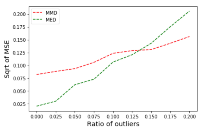
Our preprint on MMD-estimation and robustness study specifically the robustness properties of \(\hat{\theta}\). Namely, in Huber’s contamination model, we study in detail the dependence of \(\mathbb{E}[d(P_{\hat{\theta}},P^0)]\) with respect to \(n\), the sample size, and \(\varepsilon\), the level of contamination. Moreover, in this paper, we also extend the consistency proof to the case where the observations are not independent.
In the short paper on MMD-Bayes, we study a generalized Bayes procedure using the MMD distance:
\[ \pi(\theta|X_1,\dots,X_n) \propto \exp\left(- \eta d_k^2(P_\theta,\hat{P}_n) \right) \pi(\theta) \]
where \(\pi\) is some prior distribution and \(\eta>0\) some tuning parameter. This leads to robust Bayesian estimators.
We finally have two recent preprints on MMD-estimation in regression models and in copulas models, respectively. These models have in common that they are semi-parametric: we want to estimate a parameter that does not completely define the distribution of the data. For example, in the linear regression model \(Y_i = \left<\theta,X_i\right> + \varepsilon_i\), we usually only specify the distribution of \(\varepsilon\), say \(\mathcal{N}(0,\sigma^2)\). However, in order to use the MMD-estimator as defined above, one should also specify the distribution of the \(X_i\)’s. In [4], we propose a trick to avoid that, but the analysis becomes immediately much more complex.
[3] P. Alquier, B.-E. Chérief-Abdellatif, A. Derumigny and J.-D. Fermanian. Estimation of Copulas via Maximum Mean Discrepancy, to appear in Journal of the American Statistical Association. The paper comes with the R package: MMDCopula.
[4] P. Alquier and M. Gerber (2020). Universal Robust Regression via Maximum Mean Discrepancy. Preprint arxiv:2006.00840. We are currently working on the corresponding R package.
REFERENCES
[6] P. J. Bickel (1976). Another Look at Robustness: A Review of Reviews and Some New Developments. Scandinavian Journal of Statistics 3, 145-168.
[9] L. Devroye and G. Lugosi (2001). Combinatorial methods in density estimation. Springer.