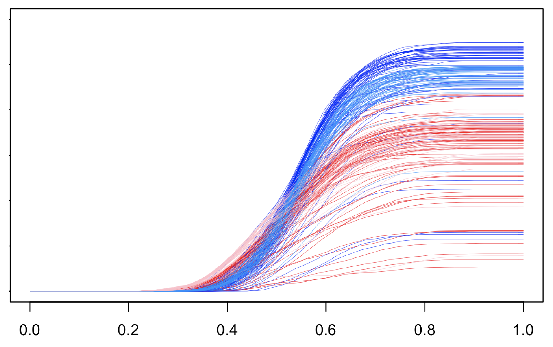
 Figure 1: Depth quantile functions for the wine data (d=13), class 2 vs class 3. Blue curves correspond to between class comparisons, red/pink correspond to within class comparisons.
A common technique in modern statistics is the so-called kernel trick, where data is mapped into a (usually) infinite-dimensional feature space, where various statistical tasks can be carried out. Relatedly, we introduce the depth quantile function (DQF), \(q_{ij}(\alpha)\) which similarly maps observations into an infinite dimensional space (the double index will become clear below), though in this case, these new representations of the data are functions of a one-dimensional variable \(\alpha\) which allows plotting. By construction, described below, these functions encode geometric information about the underlying data set. Consequently, we obtain a tool that permits an interpretable visualization of point cloud geometry regardless of dimension of the data. Additionally, tools from functional data analysis can now be used to solve problems (classification, anomaly detection, etc).
The primary tool used is that of Tukey’s half space depth (HSD), which provides a higher dimensional analog to the order statistics as a measure of centrality of an observation in a data set (where, for instance, the median is the most central or “deepest” point). In fact, the one dimensional version of HSD (\(D(x) = \min\{F_n(x), 1-F_n(x)\}\) with \(F_n\) the EDF) is all we need, as we consider projections of our data onto lines before computing centrality, see below.
It is known that for HSD in any dimension, the level sets \(\{x:D(x)\geq\lambda\}\) are necessarily convex, thus not conforming to the shape of the underlying density. Additionally, in high dimensions, it’s likely that most points live near the boundary of the point cloud (the convex hull), i.e. we expect almost all points to be “non-central”. To get around this second problem, we instead consider, for every pair of points (\(x_i, x_j\)), the midpoint \(m_{ij} = \frac{x_i + x_j}{2}\) as the base point in the construction of our feature functions \(q_{ij}(\alpha)\). Thus, we construct a matrix of feature functions, with each observation corresponding to \(n-1\) feature functions, one for every other observation in the data set (though current work uses only the average of these functions or appropriate subsets of them). The choice of the midpoint as base point is motivated as follows. Consider a 2-class modal classification problem, where each class is represented by a component of a mixture of two normal distributions for which the corresponding cluster centers (the means) are sufficiently separated. When considering a pair of observations from different classes, their midpoint is likely to live in a region between the two point clouds with few nearby observations, in other words, a low density region with a high measure of centrality. The opposite can be expected for within class comparisons, i.e. two observations from the same class.
To addresses the convexity issue alluded to above, we use “local” versions of the HSD. This is done by taking random subsets of the data space containing \(m_{ij}\) and computing the HSD for this point after projection of the subset onto the line \(\ell_{ij}\) that is determined by the two points \(x_i,x_j\). Specifically, the subsets are given by the data residing in randomly selected spherical cones of a fixed angle (which is a tuning parameter) with axis of symmetry \(\ell_{ij}\) (see figure 2.) We define a distribution of cone tips along \(\ell_{ij}\), which induces a distribution of “local” depths (HSD), and define the DQF as the corresponding quantile function of this distribution. Using directions determined by pairs of points (i.e. the lines \(\ell_{ij}\)) addresses a challenge with high dimensional data: which direction should one look to capture interesting feature of the data? It also results in this method being automatically adaptive to sparseness (data living in a lower dimensional subspace of our data space).
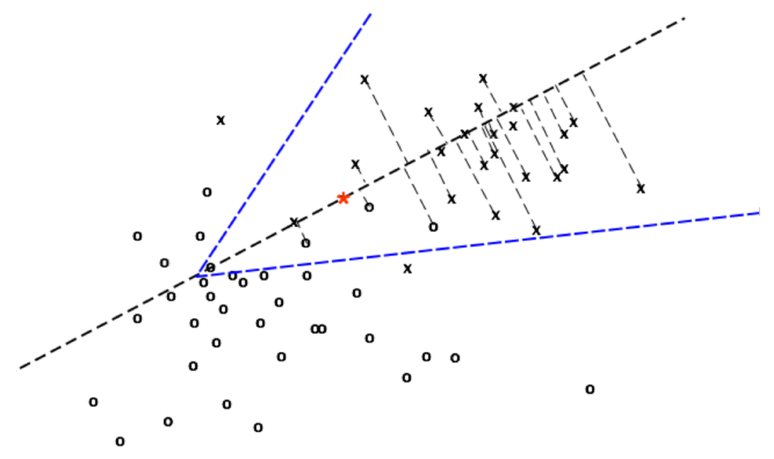 Figure 2: A local depth for midpoint in red. Depth value will be 2 for this cone tip.
As a result of this construction, we end up with a multi-scale method, a function defined on [0,1], that is non-degenerate at both boundaries (in contrast to most multi-scale methods). One can show that the derivative of \(q_{ij}(\alpha)\) as \(\alpha\to 0\) yields information about the density at \(m_{ij}\), while \(q_{ij}(1)\) is related to its centrality in the entire point cloud. The manner in which \(q_{ij}\) grows with increasing \(\alpha\), while less interpretable, yields valuable information about the observations it corresponds to.
As an example of how this information might be used, we again consider the 2-class classification problem. Each observation is described by two functions, the average function \(\frac{1}{|C_1|}\sum_{j\in C_1}q_{ij}(\alpha)\) for comparisons with class 1 (\(C_1\)), and similarly the average function for comparisons with class 2. In line with the heuristic laid out above, it can be seen in figure 1 that for an observation from class 1, comparisons with class two tends to yield functions that have low density (so are slow to grow for small quantile levels) and large value for \(\alpha=1\) corresponding to high centrality. In-class comparisons have the opposite properties. A simple heuristic for solving this classification problem might be to use the first few loadings from an fPCA and your favorite classifier for Euclidean data. Results on several data sets using an untuned SVM were competitive with existing methods with extensive tuning.
Finally, the construction only depends on the data via inner products, meaning that DQFs can be constructing on any data type for which a kernel is defined, for instance persistence diagrams in topological data analysis, allowing for a visualization of non-Euclidean data in addition to high (including infinite) dimensional Euclidean data.
Reference: Chandler, G. and Polonik, W. “Multiscale geometric feature extraction for high-dimensional and non-Euclidean data with applications.” Ann. Statist. 49 (2) 988 - 1010, April 2021. (https://arxiv.org/abs/1811.10178)