Bayesian inference

Bayesianism is about a certain interpretation of the concept probability: as degrees of belief. A Bayesian first expresses this belief as a probability function. We call this the prior distribution, and we denote it by \(\mathbb{P}(\theta)\), where \(\theta\) is the parameter (or several parameters) of the model. After the specification of the prior, we obtain the data \(D\) and the likelihood \(\mathbb{P}(D | \theta)\). Now we can compute the posterior distribution \(\mathbb{P}(\theta | D)\) with the help of Bayes’ theorem: \[\begin{aligned} \mathbb{P}(\theta | D) = \frac{\mathbb{P}(D | \theta) \mathbb{P}(\theta)}{\mathbb{P}(D)}.\end{aligned}\] Suppose we want to test a null hypothesis \(\mathcal{H}_0\) against an alternative hypothesis \(\mathcal{H}_1\). We can do this in a Bayesian way with Bayes factors: we start with the prior odds \(\mathbb{P}(\mathcal{H}_1) / \mathbb{P}(\mathcal{H}_0)\), our belief before seeing the data. Often we believe that both hypotheses are equally probable, then our prior odds are 1-to-1. Next we gather our data \(D\), and update our odds with the new knowledge, using Bayes’ theorem: \[\begin{aligned} \text{posterior odds}(\mathcal{H}_1 \text{ vs. } \mathcal{H}_0) = \frac{\mathbb{P}(\mathcal{H}_1 | D)}{\mathbb{P}(\mathcal{H}_0 | D)} = \frac{\mathbb{P}(\mathcal{H}_1)}{\mathbb{P}(\mathcal{H}_0)} \frac{\mathbb{P}(D | \mathcal{H}_1)}{\mathbb{P}(D | \mathcal{H}_0)}.\end{aligned}\] The posterior odds is our updated belief about which hypothesis is more likely.

Three notions of optional stopping

Validity under optional stopping is a desirable property of hypothesis testing: we gather some data, look at the results, and decide whether we stop of gather some additional data. Informally, we call ‘peeking at the results to decide whether to collect more data’ optional stopping, but if we want to make more precise what it means if we say that a test can handle optional stopping, it turns out that different approaches (frequentist, subjective Bayesian and objective Bayesian) lead to different interpretations and definitions. It tuns out that we can discern three main mathematical concepts of handling optional stopping, which we identify and formally define in the paper (Hendriksen, de Heide, and Grünwald 2020).
The first concept we call subjective Bayesian optional stopping or \(\tau\)-independence. If one considers a purely subjective Bayesian setting, appropriate if one truly believes one’s prior, then Bayesian updating from prior to posterior is not affected by the employed stopping rule: one ends up with the same posterior if one had decided the sample size \(n\) in advance, or if it had been determined, for example, because one was satisfied with the result at this \(n\). In this sense a subjective Bayesian procedure does not depend on the stopping rule.
The second sense of optional stopping we call calibration. As (Jeffrey N. Rouder 2014) writes: ‘If a replicate experiment yielded a posterior odds of 3.5-to-1 in favor of the null, then we expect that the null was 3.5 times as probable as the alternative to have produced the data.’ In more mathematical language, this can be expressed as \[\begin{aligned} \text{post-odds} (\mathcal{H}_1 \text{ vs. } \mathcal{H}_0 | ``\text{post-odds} (\mathcal{H}_1 \text{ vs. } \mathcal{H}_0 | D ) = a") = a.\end{aligned}\] We say this equation expresses calibration of the posterior odds. It turns out that this calibration fails to hold if one does not adhere to a purely subjective Bayesian view, in particular, it does not hold for the default priors the Bayesian psychology community is advocating (Wagenmakers 2007; J. N. Rouder et al. 2012). To get a first idea of one of the issues: default priors sometimes depend on the data. Then it is unclear what optional stopping really means, because if, using prior \(P_1(\theta)\) based on a sample of size \(n\), one had stopped at sample size \(n'< n\), one should have really used prior \(P'_1(\theta)\) based on sample of size \(n'\)…but then one would have stopped at yet another sample size \(n''\), and so on. See our paper (De Heide and Grünwald 2020) for an extensive discussion and many examples.

The third sense is a frequentist interpretation of handling optional stopping, which is about controlling the Type I error of an experiment. A Type I error occurs when we reject the null hypothesis when it is true, also called false positive. The frequentist interpretation of handling optional stopping is that the Type I error guarantee holds if we do not determine the sampling plan — and thus the stopping rule — in advance, but we may stop when we see significant results. In the case \(\mathcal{H}_0\) is simple (containing just one hypothesis), there is a well-known intriguing connection between Bayes factors and Type I error probabilities: if we reject \(\mathcal{H}_0\) iff the posterior odds in favor of \(\mathcal{H}_0\) are smaller than some fixed level \(\alpha\), then we are guaranteed a Type I error of at most \(\alpha\). And interestingly, this holds not just for fixed sample sizes but even under optional stopping. However, for composite \(\mathcal{H}_0\) this does not continue to hold. Except for the special case where all free parameters in \(\mathcal{H}_0\) are nuisance parameters observing a group structure and equipped with the corresponding right-Haar prior, and are shared with \(\mathcal{H}_1\), as we prove in (Hendriksen, de Heide, and Grünwald 2020). But for general priors and composite \(\mathcal{H}_0\), this is typically not the case.

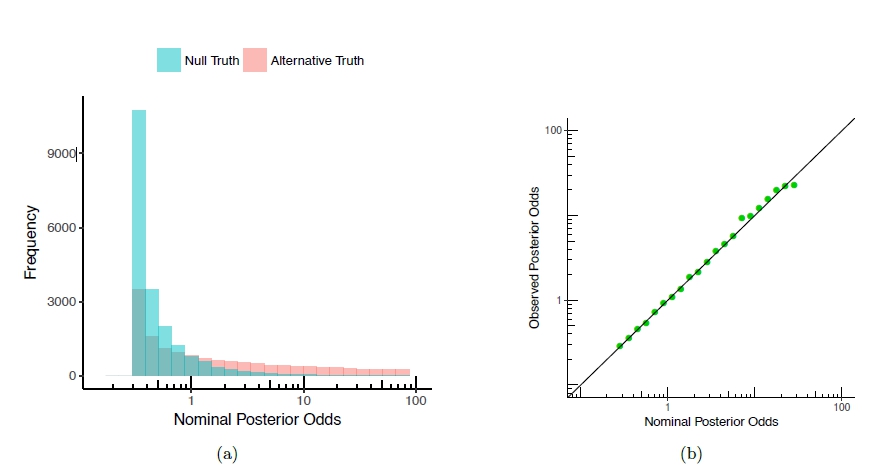
Figure 1: Posterior odds in an experiment of testing whether the mean of a normal distribution is 0 (\(\mathcal{H}_0\)), versus non-zero (\(\mathcal{H}_1\)), from 20; 000 replicate experiments. (a) The empirical sampling distribution of the posterior odds as a histogram under \(\mathcal{H}_0\) (blue) and \(\mathcal{H}_1\) (pink). (b) Calibration plot: the observed posterior odds as a function of the nominal posterior odds.

Conclusion

One can give three distinct mathematical meanings to the notion of optional stopping. Whether or not we can say that ‘the Bayes factor method can handle optional stopping’ in practice is a subtle matter, depending on the specifics of the given situation: what models are used, what priors, and what is the goal of the analysis.

References