Introduction
In the past decades, intelligent transportation system (ITS) has brought advanced technology that enables a data-rich environment and unprecedented opportunities for traffic prediction, which is considered as one of the most prevalent issues facing ITS (Li et al., 2015). We discuss the online prediction of the origin-destination (OD) demand count in traffic networks, which represents the number of trips between certain combinations of an origin and a destination. The study of OD demand prediction based on count data has a growing impact on many traffic control and management policies (Ashok, 1996, Ashok and Ben-Akiva, 2002, Li, 2005, Hazelton, 2008, Shao et al., 2014). For example, dynamic OD demand prediction is critical in planning for the charging services of the electrical vehicles (EV; Zhang et al., 2017). A well-designed charging facility network is necessary to extend the vehicle range and popularize the use of EVs. In particular, the dynamic demand between nodes of the traffic network plays a key role in determining the availability of the charging facilities, planning the multi-period charging schedules, and meeting the customer needs at the maximum extent (Zhang et al., 2017, Brandstatter et al., 2017). The objective of this study is to appropriately model the stochastic OD traffic demand counts considering the spatiotemporal correlations between different routes and epochs, while incorporating physical knowledge of the traffic network in the estimation. The estimation results are expected to enhance the prediction accuracy and robustness of the online traffic demand prediction for future epochs.
Model and method
We investigate a multivariate Poisson log-normal model with a block-diagonal covariance matrix and incorporate domain knowledge of the traffic network features to account for spatial correlations. Let \(N_{\text{ijt}}\) denote the observed traffic demand (i.e., the count of vehicles) for route \(j\) on day \(i\), at epoch \(t\). Based on the natural characteristics of the demand counts, it is reasonable to model each observation \(N_{\text{ijt}}\) with a Poisson log-linear model (Perrakis et al., 2014, Xian et al. 2018) such that
\[N_{\text{ijt}}\sim\text{Poisson}\left( \lambda_{\text{ijt}} \right),u_{\text{ijt}} = \log\lambda_{\text{ijt}}.\]
Here \(\lambda_{\text{ijt}}\) is the intensity of the Poisson process, and \(u_{\text{ijt}}\) is the log transformation of the intensity. To characterize the spatiotemporal correlations across different routes and time points, we model \(u_{\text{ijt}}\) as a mixed-effect Gaussian process based on \(K\) basis functions \(B_{k}(t)\) that
| \[u_{\text{ijt}} = \mu_{\text{jt}} + \sum_{k = 1}^{K}{\gamma_{\text{jk}}B_{k}(t)} + Z_{\text{ijt}}.\] \(1\) |
Here \(\mathbf{\mu =}\left\lbrack \mu_{11},\mu_{12},\ \cdots,\ \mu_{\text{JT}} \right\rbrack\mathbf{'}\) is the fixed effect coefficient that models the common characteristics of the whole traffic network, and \(\mathbf{\gamma}_{k}\mathbf{=}\left\lbrack \gamma_{1k},\ \gamma_{2k},\ \cdots,\ \gamma_{\text{Jk}} \right\rbrack\) is the random effect coefficient with prior distribution \(\mathbf{\gamma}_{k}\sim N(0,\ \mathbf{R}_{\theta_{y}})\) that characterizes the uniqueness of different routes. Here \(\mathbf{R}_{\theta_{y}}\) is the correlation matrix which takes into consideration of the traffic network information, where \(\left\lbrack \mathbf{R}_{\theta_{y}} \right\rbrack_{j_{1},j_{2}} = \sigma_{j_{1},\ j_{2}}\exp\left\{ - \theta_{y}\left| \mathbf{y}_{j_{1}} - \mathbf{y}_{j_{2}} \right|^{2} \right\}\). In this expression, \(\mathbf{y}_{j}\) denotes the unique features of route \(j\), such as information about the origin and destination, the maximum speed limit on a route, and the travel distance. The term \(Z_{\text{ijt}}\) in model (1) is the random error that follows a Gaussian distribution which has the covariance structure
| \[\text{cov}\left( Z_{ij_{1}t_{1}},Z_{ij_{2}t_{2}} \right) = \sigma_{j_{1},\ j_{2}}\exp\left\{ - \theta_{y}\left| \mathbf{y}_{j_{1}} - \mathbf{y}_{j_{2}} \right|^{2} \right\} \cdot \tau^{2}\exp\left\{ - \theta_{t}\left| t_{1} - t_{2} \right| \right\}.\] \(2\) |
Which depends on both the features of routes \(j_{1}\) and \(j_{2}\), and the time points \(t_{1}\) and \(t_{2}\), which we refer to as the spatial and temporal covariance structures, respectively.
Denote the log-transformed intensity of the OD traffic demand on day \(i\) as \(\mathbf{u}_{i} = \left( u_{i11},u_{i12},\ldots,u_{\text{iJT}} \right)^{'}\). We can further derive that conditioning on parameters \(\left( \mathbf{\mu},\ \theta_{y},\theta_{t},\mathbf{\sigma,\ }\tau^{2} \right)\), \(\mathbf{u}_{i}\) follows normal distribution \(N\left( \mathbf{\mu},\ \mathbf{\Sigma} \right)\), where
\[\mathbf{\mu} = \left( \mu_{11},\mu_{12},\ \cdots,\ \mu_{\text{JT}} \right)^{'},\]
| \[\mathbf{\Sigma} = \mathbf{R}_{\theta_{y}}\bigotimes\left\lbrack \mathbf{R}_{B} + \tau^{2}\mathbf{R}_{\theta_{t}} \right\rbrack.\] \(3\) |
Here, the symbol \(\bigotimes\) denotes the Kronecker product, \(\mathbf{R}_{B}\) is a fixed \(T \times T\) matrix with the \((t_{1},t_{2})\) element equal to \(\sum_{k = 1}^{K}{B_{k}(t_{1})B_{k}(t_{2})}\), and \(\mathbf{R}_{\theta_{t}}\) is a \(T \times T\) matrix with the \((t_{1},t_{2})\) element equal to \(\exp\left\{ - \theta_{t}|t_{1} - t_{2}| \right\}\). Therefore, the large covariance matrix is parametrized based on only the parameters \(\theta_{y},\theta_{t},\mathbf{\sigma}\), and \(\tau^{2}\). This parsimonious model has several advantages, such as high interpretability tailored to the traffic demand count data, increased stability of the estimation results, and reduced computational burden for parameter estimation. We treat \(\mathbf{u}\) as a latent variable and further employ the EM algorithm to obtain the maximum likelihood estimation (MLE) for the parameters.
In this way, we can fully explore the complicated spatiotemporal correlation structure of the traffic network demand and automatically cluster the routes with high correlations, without introducing a large number of parameters that impact the estimation accuracy. Besides transportation systems, the proposed method can be easily extended to other network applications with count data through few modifications, such as communication systems, supply chain management, smart grid, or even three-dimensional networks (Wang et al., 2018).
Case study
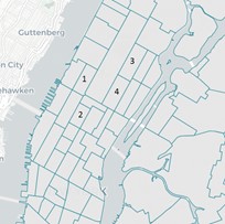
We apply the proposed method to a real New York yellow taxi dataset which is collected from June 1st to July 31st in 2017 (NYC taxi, 2017). The dataset records all yellow taxi trips during the aforementioned time period including the pick-up and drop-off dates and times, pick-up and drop-off locations, trip distances, and payment information about the trips. We focus on the trips between the four busiest zones in Manhattan and investigate the structure of the travel demand counts on these zones as OD pairs. The details of the four taxi zones are shown in Figure 1.

| Index | Borough | Zones |
|---|---|---|
| 1 | Manhattan | Lincoln Square East |
| 2 | Manhattan | Times Square/Theatre District |
| 3 | Manhattan | Upper East Side North |
| 4 | Manhattan | Upper East Side South |
Figure 1. Illustration of the taxi zones in the case study
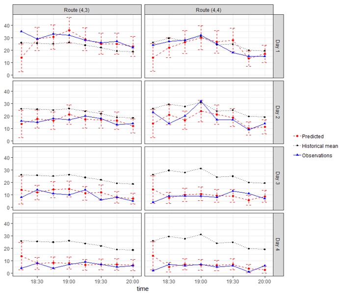
Figure 2 further shows the specific taxi demand prediction results of two routes \((4,\ 3)\) and \((4,\ 4)\) for four test days. The solid black line in this figure represents the true dynamic traffic demand counts, where it can be observed that the true taxi demand indeed exhibits high spatial and temporal variation and strong correlations for observations between the routes and across different epochs. The solid red line in is the predicted demand using the proposed method, and the dashed error bars show the 90% confidence interval of the prediction based on the variance derivation in equation (7), which significantly outperforms the existing method shown in black dotted line.

Figure 2. Taxi demand prediction results for routes \((4,\ 3)\) and \((4,\ 4)\).
This post is based on
Xian, X., Ye, H., Wang, X., and Liu, K. (2021). Spatiotemporal modeling and real-time prediction of origin-destination traffic demand. Technometrics, 63(1), 77-89.
References
- Li, L., Su, X., Zhang, Y., Lin, Y., and Li, Z. (2015). Trend modeling for traffic time series analysis: An integrated study. IEEE Transactions on Intelligent Transportation Systems, 16(6), 3430-3439.
- Ashok, K. (1996). Estimation and prediction of time-dependent origin-destination flows (Doctoral dissertation, Massachusetts Institute of Technology).
- Ashok, K., and Ben-Akiva, M. E. (2002). Estimation and prediction of time-dependent origin-destination flows with a stochastic mapping to path flows and link flows. Transportation Science, 36(2), 184-198.
- Brandstatter, G., Kahr, M., and Leitner, M. (2017). Determining optimal locations for charging stations of electric car-sharing systems under stochastic demand. Transportation Research Part B: Methodological, 104, 17-35.
- Li, B. (2005). Bayesian inference for origin-destination matrices of transport networks using the EM algorithm. Technometrics, 47(4), 399-408.
- Hazelton, M. L. (2008). Statistical inference for time varying origin–destination matrices. Transportation Research Part B: Methodological, 42(6), 542-552. NYC taxi, (2017). Retrieved from http://www.nyc.gov/html/tlc/html/about/trip_record_data.shtml.
- Perrakis, K., Karlis, D., Cools, M., Janssens, D., Vanhoof, K., and Wets, G. (2012). A Bayesian approach for modeling origin-destination matrices. Transportation Research Part A: Policy and Practice, 46(1), 200-212.
- Shao, H., Lam, W. H., Sumalee, A., Chen, A., and Hazelton, M. L. (2014). Estimation of mean and covariance of peak hour origin-destination demands from day-to-day traffic counts. Transportation Research Part B: Methodological, 68, 52-75.
- Wang, D., Liu, K., and Zhang, X. (2018), “Modeling of a three-dimensional dynamic thermal field under grid-based sensor networks in grain storage”, in press, IISE Transactions.
- Zhang, A., Kang, J. E., and Kwon, C. (2017). Incorporating demand dynamics in multi-period capacitated fast-charging location planning for electric vehicles. Transportation Research Part B: Methodological, 103, 5-29.
About the authors
 Dr. Xiaochen Xian is an assistant professor from the Department of Industrial and Systems Engineering at the University of Florida.
 Honghan Ye is a Ph.D. candidate from the Department of Industrial and Systems Engineering at UW-Madison.
 Dr. Xin Wang is an assistant professor from the Department of Industrial and Systems Engineering at UW-Madison.
 Dr. Kaibo Liu is an associate professor from the Department of Industrial and Systems Engineering at UW-Madison.