Overview of the method

The objective of GANs is to randomly generate artificial contents similar to some data. Put another way, they are aimed at sampling according to an unknown distribution \(P^\star\), based solely on i.i.d. observations \(X_1, \dots, X_n\) drawn according to \(P^\star\). Obviously, a naive approach would be to:

1. Estimate the distribution \(P^\star\) by some \(\hat P\).
2. Sample according to \(\hat P\).

However, both tasks are difficult in themselves. In particular, density estimation is made arduous by the complexity and high dimensionality of the data involved in the domain, relegating both standard parametric and nonparametric approaches unworkable. Thus, GANs offer a completely different way to achieve our goal, often compared to the struggle between a police team, trying to distinguish true banknotes (the observed data \(X_1, \dots, X_n\)) from false ones (the generated data), and a counterfeiters team (the generator), slaving to produce banknotes as credible as possible and to mislead the police.

To be a bit more specific, there are two brilliant ideas at the core of GANs:

1. Sample data in a very straightforward manner thanks to the transform method: let \(\mathscr G=\left \{G_{\theta}: \mathbb R^\ell \to \mathbb R^d, \theta \in \Theta \right\}\), where \(\ell\) is the dimension of what is called the latent space and \(\Theta \subset \mathbb R^p\), be a class of measurable functions, called generators (in practice \(\mathscr G\) is often a class of neural networks with \(p\) parameters). Now, let us sample \(Z \sim \mathcal N(0, I_\ell)\) and compute \(U = G_\theta(Z)\). Then, \(U\) is an observation drawn according to the distribution \(P_\theta = G_\theta \# N(0, I_\ell)\) (the push-forward measure of the latent distribution \(N(0, I_\ell)\) according to \(G_\theta\)). In other words, the statistical model for the estimation of \(P^\star\) has the form \(\mathscr P = \left\{ P_\theta = G_\theta \# N(0, I_\ell), \theta \in \Theta \right\}\) and it is definitely straightforward to sample according to \(P_\theta\).
2. Assessing the proximity between \(P_\theta\) and \(P^\star\) by comparing two samples \(X_1, \dots, X_n \overset{i.i.d.}{\sim} P^\star\) and \(U_1, \dots, U_n \overset{i.i.d.}{\sim} P_\theta\). What does comparing mean? Assume the group of \(X_1, \dots, X_n\) is very difficult to ``separate’’ from the group of \(U_1, \dots, U_n\), or put another way, it is very difficult to distinguish the class of \(X_1, \dots, X_n\) from the class of \(U_1, \dots, U_n\). Would you be convinced that the two distributions \(P_\theta\) and \(P^\star\) are very close (at least for large \(n\))? That is exactly the point.

Comparing distributions

At this point, Task 2 is still a bit blurry and deserves further details about how to quantify the difficulty (or the ease) of separating the two classes \(X_1, \dots, X_n\) and \(U_1, \dots, U_n\). This problem is actually closely related to supervised learning, and in particular to classification: assume that a classifier, let us say \(h : \mathbb R^d \to \{0, 1\}\), manages to perfectly discriminate the two classes: \(\mathbb P(h(X_1)=1) = \mathbb P(h(U_1)=0) = 1\), then we can say that the two distributions \(P_\theta\) and \(P^\star\) are different. Conversely, if the classifier is fooled, that is \(\mathbb P(h(X_1)=1) = \mathbb P(h(U_1)=0) = \frac 12\), we may accept that the two distributions are identical.

This classification setting is formalized as following: let \((X, Y)\) be a pair of random variables taking values in \(\mathbb R^d \times \{0, 1\}\) such that: \[ X|Y=1 \sim P^\star \quad \text{and} \quad X|Y=0 \sim P_\theta, %\tag{M} \] and let \(\mathscr D = \left \{D_{\alpha} : \mathbb R^d \to [0, 1], \alpha \in \Lambda \right\}\), \(\Lambda \subset \mathbb R^q\), be a parametric model of discriminators such that \(D_\alpha(x)\) is aimed at estimating \(\mathbb P(Y=1 | X=x)\) (put another way, the distribution of \(Y|X=x\) is estimated by \(\mathcal B(D_\alpha(x))\)). For a given discriminator \(D_\alpha\), the corresponding classifier is \(h : x \in \mathbb R^d \mapsto \mathbb 1_{D_\alpha(x) > \frac 12}\).

The sample \(\{ (X_1, 1), \dots, (X_n, 1), (U_1, 0), \dots, (U_n, 0) \}\), previously build by putting together observed and generated data, fits the classification model and can serve for estimating a classifier by maximizing the conditional log-likelihood: \[ \hat \alpha \in \operatorname*{arg\,max}_{\alpha \in \Lambda} \hat L(\theta, \alpha), \quad \text{where} \quad \hat L(\theta, \alpha) = \frac 1n \sum_{i=1}^n \log(D_\alpha(X_i)) + \frac 1n \sum_{i=1}^n \log(1-D_\alpha(U_i)). \] In addition, the maximal log-likelihood \(\sup_{\alpha \in \Lambda} \hat L(\theta, \alpha)\) reflects exactly the ease of discrimination of the two classes \(X_1, \dots, X_n\) and \(U_1, \dots, U_n\), that is the proximity between \(P_\theta\) and \(P^\star\). Task 2 is thus performed by introducing a class of discriminators (which are often neural networks) and maximizing a log-likelihood. The latter quantity also helps in adjusting \(\theta\) such that the distribution \(P_{\theta}\) of the generated data \(G_\theta(Z)\) becomes closer and closer to \(P^\star\).

In statistical terms, \(P^\star\) can be estimated by \(P_{\hat \theta}\), where: \[ \hat \theta \in \operatorname*{arg\,min}_{\theta \in \Theta} \sup_{\alpha \in \Lambda} \hat L(\theta, \alpha), \] where, as described previously, the generated data is \(U_i = G_\theta (Z_i)\) with \(Z_1, \dots, Z_n \overset{i.i.d.}{\sim} \mathcal N(0, I_\ell)\).

The story of GANs is not that gleaming since, in practice, we never have access to \(P_{\hat \theta}\), which may be a very complicated object, but only to the generator \(G_{\hat \theta}\). Anyway, our aim is to sample according to \(P^\star\), which can be achieved (up to the estimation error) thanks to \(G_{\hat \theta}(Z)\), where \(Z \sim \mathcal N(0, I_\ell)\).

Actually, in this work, \(P_\theta\) is just as a mathematical object helping to understand GANs. To go into details, the forthcoming results are based on the assumption that all distributions in play are absolutely continuous with respect to a known measure \(\mu\) (typically the Hausdorff measure on some submanifold of \(\mathbb R^d\)) and probability density functions are noted with lowercase letters (in particular \(P^\star = p^\star d\mu\) and \(P_\theta = p_\theta d\mu\)).

Concerning the comparison of distributions

In order to give a mathematical foundation to our intuition in Task 2, it may be useful to analyze the big sample case, where \[\hat L(\theta, \alpha) \approx \mathbb E [\hat L(\theta, \alpha)] = \mathbb E [\log(D_\alpha(X_1))] + \mathbb E [\log(1-D_\alpha\circ G_\theta(Z_1))].\]

If the class of discriminators \(\mathscr D = \left\{ D_\alpha, \alpha \in \Lambda \right\}\) is rich enough to contain the ``optimal’’ discriminator \(D_\theta^\star = \frac{p^\star}{p_\theta + p^\star}\) for all \(\theta \in \Theta\), then \[\sup_{\alpha \in \Lambda} \mathbb E [\hat L(\theta, \alpha)] = 2 D_{JS}(P^\star, P_\theta) - \log 4,\] where \(D_{JS}\) is the Jensen-Shannon divergence (Endres and Schindelin 2003).

Two things can be learned from this first result (still assuming that \(\mathscr D\) contains ``optimal’’ discriminators):

1. Up to the approximation capacity of \(\mathscr D\), \(\sup_{\alpha \in \Lambda} \hat L(\theta, \alpha)\) does reflect the proximity between \(P_\theta\) and \(P^\star\) (thanks to an approximated divergence).
2. \(\hat \theta\) cannot be better than \(\theta^\star \in \operatorname*{arg\,min}_{\theta \in \Theta} \sup_{\alpha \in \Lambda} \mathbb E [\hat L(\theta, \alpha)] = \operatorname*{arg\,min}_{\theta \in \Theta} D_{JS}(P^\star, P_\theta)\), which leads to the approximation \(P_{\theta^\star}\) of \(P^\star\) obtained by minimizing the Jensen-Shannon divergence.

Non-asymptotic bound on Jensen-Shannon error

Thus, GANs drive the world downhill in two directions:

1. A limited approximation capacity for the class of discriminators \(\mathscr D\) (which may not contain the ``optimal’’ discriminator \(D_\theta^\star = \frac{p^\star}{p_\theta + p^\star}\) for all \(\theta \in \Theta\)): \(\sup_{\alpha \in \Lambda} \mathbb E [\hat L(\theta, \alpha)] < 2 D_{JS}(P^\star, P_\theta) - \log 4\).
2. A finite sample approximation: the criterion maximized is \(\hat L(\theta, \alpha)\) instead of \(\mathbb E [\hat L(\theta, \alpha)]\).

These limitations introduce two kinds of error in the estimation procedure: an approximation error (or bias), induced by the richness of \(\mathscr D\), and an estimation error (or variance) occurring from the finiteness of the sample.

This can be formalized in the following manner: assume some regularity conditions of the first order on the models \(\mathscr P\), \(\mathscr G\) and \(\mathscr D\) and assume that optimal discriminators \(D_\theta^\star\) can be approximated by \(\mathscr D\) up to an error \(\epsilon>0\) in \(L^2\)-norm. Then: \[ \mathbb E [D_{JS}(P^\star, P_{\hat \theta})] - D_{JS}(P^\star, P_{\theta^\star}) = O \left( \epsilon^2 + \frac{1}{\sqrt n} \right). \]

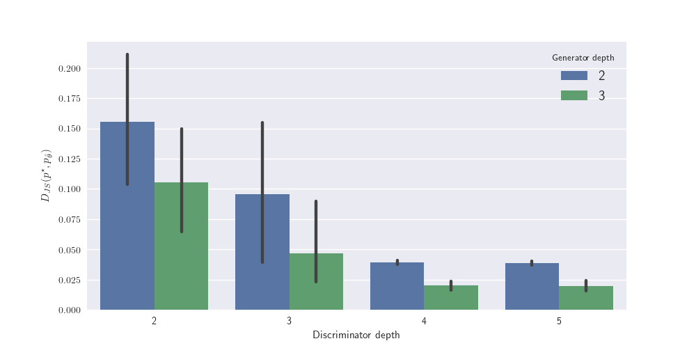
This result explains quantitatively that the discriminators in GANs have to be tuned carefully: on the one hand, poor discriminators induce an uncontrolled gap between \(\sup_{\alpha \in \Lambda} \mathbb E [\hat L(\theta, \alpha)]\) and \(D_{JS}(P^\star, P_\theta)\); on the other hand, very flexible discriminators may lead to overfitting the finite sample.

The first assertion is illustrated in the next figure. The numerical experiment has been set up with classes of fully connected neural networks for the generators and the discriminators (respectively \(\mathscr G\) and \(\mathscr D\)) and \(n\) sufficiently large. The depth of the generators is either 2 (blue bars) or 3 (green bars) and the depth of the discriminator ranges from 2 to 5 (from left to right). As expected, it appears clearly that the more flexible the discriminators are (from left to right), the smaller \(D_{JS}(P^\star, P_{\hat \theta})\) is. Obviously, this is also inversely correlated with the richness of the class of generators \(\mathscr G\) (at least in a first regime).

Asymptotic normality

As a second important result, it can be shown that the estimator \(\hat \theta\) is asymptotically normal with convergence rate \(\sqrt n\). More formally, let us assume \(\bar \theta \in \operatorname*{arg\,min}_{\theta\in\Theta} \sup_{\alpha \in \Lambda} \mathbb E [\hat L(\theta, \alpha)]\) exists and is unique. Let also assume some regularity conditions of the second order on the models \(\mathscr P\), \(\mathscr G\) and \(\mathscr D\), well definiteness and smoothness of \(\theta \mapsto \operatorname*{arg\,max}_{\alpha \in \Lambda} \mathbb E [\hat L(\theta, \alpha)]\) around \(\bar \theta\). Then, there exists a covariance matrix \(\Sigma\) such that: \[ \sqrt n \left( \hat \theta - \bar \theta \right) \xrightarrow{dist} \mathcal N(0, \Sigma). \]