Introduction
Let us start by considering the optimal rejection policy for a single hypothesis testing problem. There are three elements to the problem. The objective: to maximize the power to reject the null hypothesis. The constraint: to control the type I error probability, so that it is at most a predefined \(\alpha\). The decision policy: for every realized sample define the decision \(D\in \{0,1\}\), where the null hypothesis is rejected if \(D=1\) and retained otherwise. For simplicity, let \(z\) be the realized test statistic on which the decision \(D\) is based, and let \(g(z\mid h=1)\) and \(g(z\mid h=0)\) be, respectively, the non-null and the null density of \(z\). The optimization problem is therefore: \[\max_{D:\mathbb R \rightarrow \{0,1\}} \int D(z)g(z\mid h=1)dz\\ s.t.\int D(z)g(z\mid h=0)dz\leq \alpha. \] This infinite dimensional integer problem happens to have a simple solution provided by the Neyman-Pearson (NP) Lemma.
In this era of big data, conducting a study with a single hypothesis is rare. In many disciplines, hundreds or thousands of null hypotheses are tested in each study. In order to avoid an inflation of false positive findings, it is critical to use multiple testing procedures that guarantee that a meaningful error measure is controlled at a predefined level \(\alpha\). The most popular measures are the family wise error rate (FWER), i.e., the probability of at least one type I error, and the false discovery rate (FDR), i.e., the expected false discovery proportion.
Arguably, it is just as critical that the multiple testing procedure will have high statistical power, thus facilitating scientific discoveries. As with the single hypothesis testing problem, we take an optimization approach to the problem with \(K>1\) null hypotheses: we seek to find the \(K\) decision functions, \(\vec D: {\mathbb R}^K\rightarrow \{0,1 \}^K\), that maximize some notion of power while guaranteeing that the error measure is at most \(\alpha\). In this post, we shall consider the problem of finding the optimal decision functions when testing multiple hypotheses in a couple of settings of interest.
This post is based on our three recent papers on this topic: Rosset et al. (2018), where a general theoretical framework is presented; Heller and Rosset (2021), where the two-group model is discussed; and Heller, Krieger and Rosset (2021), where optimal clinical trial design is discussed.
An optimal policy for the two-group model
The two-group model, which is widely used in large scale inference problems, assumes a Bayesian setting, where the observed test statistics are generated independently from the mixture model \[(1-\pi)g(z\mid h=0)+\pi g(z\mid h=1),\] where \(h\) follows the \(Bernoulli(\pi)\) distribution, and indicates as before whether the null is true \((h=0)\) or false \((h=1)\). Let \(\vec z\) be a vector of length \(K\) generated according to the two group model, and consider the following optimization problem: \[\max_{\vec D:{\mathbb R}^K \rightarrow \{0,1\}^K} \mathbb E(\vec h^t \vec D) \\ s.t. \ FDR(\vec D) \leq \alpha.\] One of our main results is that the solution is to threshold the test statistic \[\mathbb P(h=0\mid z) = \frac{(1-\pi)g(z\mid h=0)}{(1-\pi)g(z\mid h=0)+\pi g(z\mid h=1)}, \] and that the threshold depends on the entire vector of test statistics \(\vec z\). Thus for a realized vector of test statistics \(\vec z = (z_1, \ldots, z_K)\), the decision vector \(\vec D\) can be described in the following form: \[\vec D(\vec z) = (\mathbb I[\mathbb P(h=0\mid z_1)\leq t(\vec z)], \ldots, \mathbb I[\mathbb P(h=0\mid z_k)\leq t(\vec z)]),\] where \(\mathbb I[\cdot]\) is the indicator function. This leads to practical algorithms which improve theoretically and empirically on previous solutions for the two-group model.
An optimal policy for the design of clinical trials
Assume that \(K=2\) hypothesis testing problems are examined in a clinical trial (e.g., treatment effectiveness in two distinct subgroups). The federal agencies that approve drugs typically require strong FWER control at level \(\alpha = 0.05\). At the design stage, it is necessary to decide on the number of subjects that will be allocated. For \(K=1\), this is typically done by computing the minimal number of subjects for achieving minimal power with a type I error probability of \(\alpha\). For \(K=2\), with a relevant notion of required power \(\Pi(\vec D)\), a smaller number of subjects will need to be allocated, if the multiple testing procedure is the optimal policy, rather than an off-the-shelf policy. However, finding the optimal policy may be difficult since the policy has to guarantee that for every data generation with at least one null parameter value, the probability of rejecting the null hypothesis corresponding to the null parameter value should be at most \(\alpha\) (i.e., there may be an infinite number of constraints for strong FWER control at level \(\alpha\)).
For simplicity, assume we have two independent test statistics that are normally distributed with variance one and expectation zero if the null hypothesis is true but negative if the null hypothesis is false. Then, the optimization problem can be formalized as follows:
\[\max_{\vec D:{\mathbb R}^2 \rightarrow \{0,1\}^2} \Pi(\vec D) \\ s.t. \ \mathbb P_{(0, \theta)}(D_1=0) \leq \alpha \ \forall \ \theta <0; \ \mathbb P_{( \theta, 0 )}(D_2=0) \leq \alpha \ \forall \ \theta <0; \ \mathbb P_{(0, 0)}(\max(D_1,D_2)=0) \leq \alpha.\]
We also add the common-sense restriction that \(p\)-values above \(\alpha\) are not rejected (for details, see Heller, Krieger, and Rosset 2021).
The resulting optimal rejection policy is attractive for relevant objectives \(\Pi(\vec D)\) that can be useful for clinical trials.
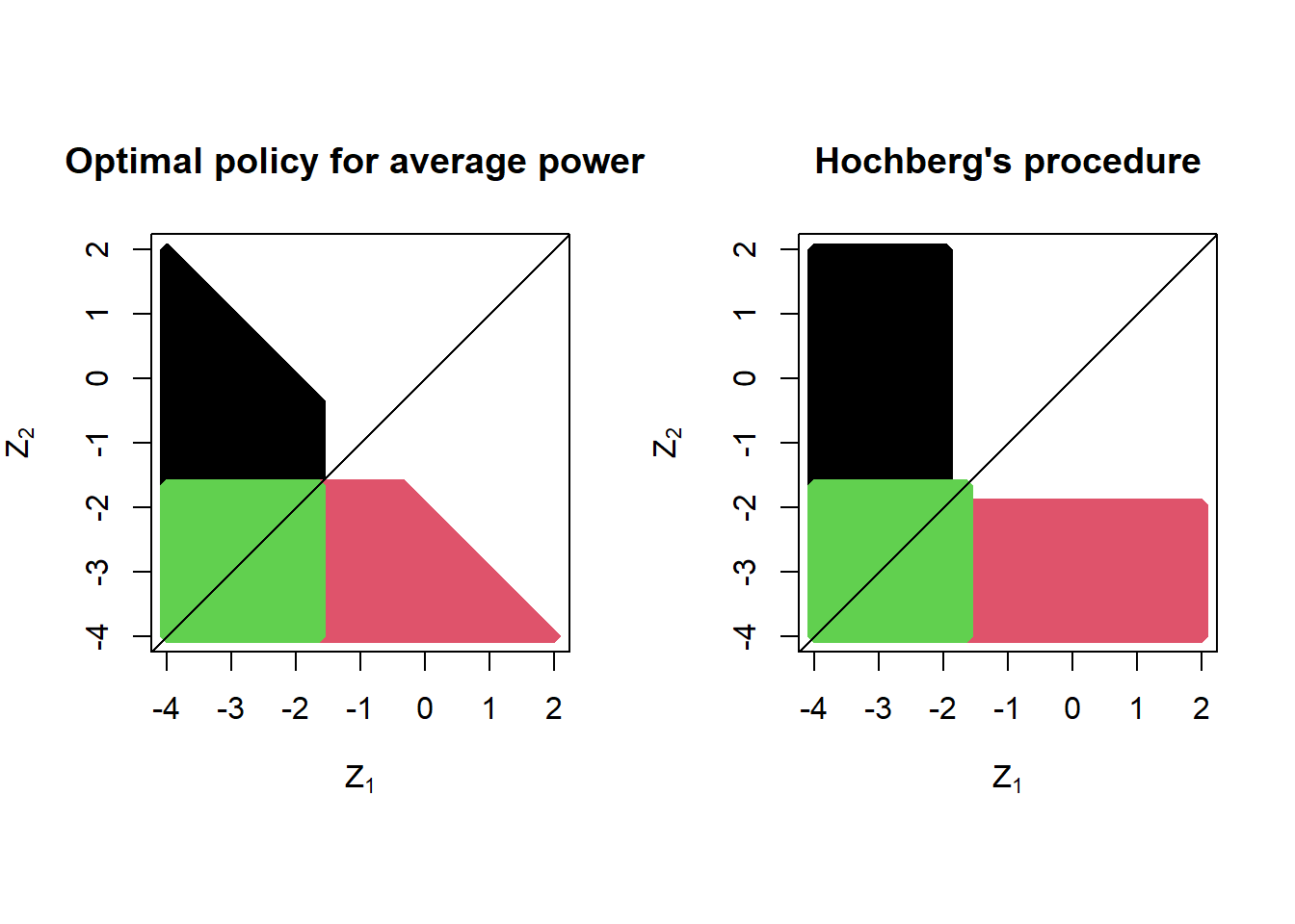
Below we provide one example optimal policy: the policy maximizing the average power when both test statistics have expectation -2 (left panel). For comparison, we provide the off-the-shelf popular Hochberg procedure (which coincides with the Hommel procedure for \(K=2\)). Both policies satisfy the strong FWER control guarantee at level \(\alpha = 0.05\), but the average power of the optimal policy is 3% higher (63% versus 60%) if the test statistics are normally distributed with expectation -2. The color coding is as follows: in red, reject only the second hypothesis; in black, reject only the first hypothesis; in green, reject both hypotheses.

This post is based on
Heller, R. Krieger, A. and Rosset, S. (2021) Optimal multiple testing and design in clinical trials. arXiv:2104.01346
Heller, R. and Rosset, S. (2020) Optimal control of false discovery criteria in the two-group model. Journal of the Royal Statistical Society, Series B, https://doi.org/10.1111/rssb.12403
Rosset, S. Heller, R. Painsky, A. and Aharoni, E. (2018) Optimal and Maximin Procedures for Multiple Testing Problems. arXiv: 1804.10256

