Compositional scalar-on-function regression as a tool (not only) for geological data

Functional regression model

First, take a look at the standard functional data analysis (FDA) approach which was developed for functions from \(L^2\) space. A functional linear regression model with functional predictor is built as \[ y_{i} = \beta_{0} + \int_{I} \beta_{1}(t)f_{i}(t)dt + \epsilon_{i},\quad i=1,\dots,N,\quad t \in I \] where \(\beta_{0}\) is the scalar intercept and \(\beta_{1}\) represents the functional regression parameter. This model can be seen as an extension of the multiple regression - therefore, the estimators \(\hat{\beta_{0}}\) and \(\hat{\beta_{1}}\) minimize the following sum of squared errors (SSE) \[ \text{SSE} (\beta_{0},\beta_{1}) = \sum_{i=1}^{N}\left(y_{i}-\beta_{0}-\int_{I}\beta_{1}(t)f_{i}(t)dt\right)^2. \] Unfortunately, it is not common for functional data to be available in its continuous form - we are usually left with dicrete observations. To represent the sparsely measured data as functions, a proper basis expansion for both the predictors and \(\beta_{1}\) is necessary. This way, a reduction to a multivariate problem can be achieved. Furthermore, it is useful to apply the results of functional principal component analysis (FPCA) to project the data into a lower-dimensional space.

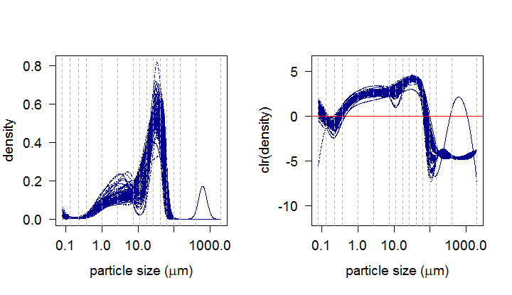
But how can we use these ideas and adapt them for the situation where the covariate consists of density functions? As each PSD forms a probability density function on the considered support, specific properties of densities (scale invariance, relative scale, unit integral) prevent from using standard FDA methods directly to PSDs. Instead, we acknowledge the possibility to represent density functions in the Bayes space \(\mathcal{B^2}\) with square-integrable log-densities as they can be then adequately represented in the \(L^2\) space due to the isomorphism between \(\mathcal{B^2}\) and \(L^2\). Frequently, the centered log-ratio (clr) transformation \[ \text{clr}(f)(t):=f_{c}(t)= \text{ln} f(t) - \frac{1}{\eta}\int_{I}\text{ln}f(t) dt \] is used to the original densities with \(\eta\) representing the length of their common (bounded) support \(I\). It can be shown that the clr transformation of densities enforces the resulting functions to integrate on \(I\) to 0. To represent the original data in continuous form while fulfilling the zero integral constraint, the so-called compositional splines were developed (more on this in Machalová et al. (2020)) and used throughout the regression modeling.

In our geological example, 96 soil samples from loesses are examined and the task is to analyze how the geochemistry of the samples is influenced by their PSDs. The cubic polynomials were chosen for the spline basis of the PSDs together with 16 knots represented in the graphs by the grey dashed lines. The resulting clr densities are now ready to serve as predictor in our regression model. For the response, the clr-transformed geochemical compositions of the observed soil samples are taken into consideration. In this case, each composition is characterized by a real vector consisting of concentrations of 9 elements (Al, Si, K, Ca, Fe, As, Rb, Sr, Zr).

Compositional regression

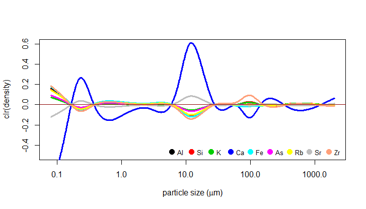
As mentioned above, the FPCA is a useful technique here to filter out noise which could distort the regression estimates - the FPCA allows us to represent the predictor using only a few functional principal components while explaining a substantial percentage of the variability of the original data. In this case, 3 principal components were used as they explained over 90% of the variability. The regression modeling is then performed on these functional principal components. The resulting functional parameters \(\beta_{1}\) are shown in the plot below (in their clr form, of course).

Quality of the model, interpretation

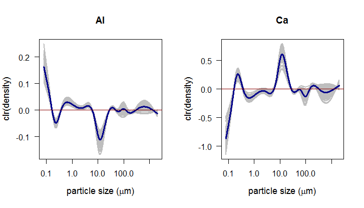
To assess the goodness-of-fit of the regression model, standard coefficient of determination can be computed with values close to one indicating a good fit of the model. Another possibility is to use a nonparametrical method of bootstrap confidence bands. The idea of bootstrap bands is based on resampling the residuals - for each part of the composition, the residuals can be estimated as \[ \hat{\epsilon}_{i}=y_i-\hat{y}_i. \] By resampling we are able to compute an arbitrary number of bootstrap samples \[ y_{i}^{boot}=\beta_{0}+\int_{I}\beta_{1}(t)\cdot f_{i}(t)dt + \epsilon_{i}^{boot},\quad i=1,\dots,N, \] and the resulting bootstrap estimates of the functional regression parameter then form a band “around” \(\beta_{1}\). Here, 100 bootstrap functions were plotted together with the estimate of \(\beta_{1}\). The bootstrap bands appear to be very useful for interpretation of the functional parameters \(\beta_{1}\) as shown for Al and Ca bellow.

While sticking with the clr form of \(\beta_{1}\) (further as clr(\(\beta_{1}\))) and their zero integral constraint, the functions have to cross the x-axis meaning that we are able to split the original support \(I\) on subdomains where clr(\(\beta_{1}\)) is positive or negative, respectively. The same can be said about the clr transformation of the particle size distributions. For interpretation, we look at the positive and negative subdomains individually. For subdomain where the clr transformed PSDs are positive (\(I^{+}\)), three situations may occur:

• the estimated parameter clr(\(\beta_{1}\)) is positive - in that case, we can expect an increasing relative presence of the given element within the geochemical composition (by considering intepretation of the clr representation of this element).

• clr(\(\beta_{1}\)) is negative, resulting in decreasing relative presence.

• clr(\(\beta_{1}\)) \(\approx 0\), meaning that the relative presence of the given element within the geochemical composition is not influenced by the respective particle sizes of the PSDs. The bootstrap confidence bands can be used to define these subdomains.

Clearly, the opposite would apply for the subdomain with negative clr transformed PSDs (\(I^{-}\)). In case of Al it means that its relative presence in the composition is strongly (positively) influenced by the finest fractions and there is also a stronger negative effect of the fraction around 10 \(\mu m\). For Ca completely opposite effects can be observed.

To sum up, the specific properties of compositional data (as multivariate data) and probability density functions (as functional data) need a proper adaptation of standard statistical methods. Here, the linear regression was addressed by presenting a compositional scalar-on-function regression model with functional predictor and real response. Hopefully the presented example demonstrated that the compositional approach with the clr transformation not only provides an adequate platform for working with probability densities, but also leads to an easier and more straight-forward interpretation of the resulting parameters.