Abstract
Binary classification is one of the cornerstones of modern data science, but, until recently, our understanding of classical methods such as the k-nn algorithm was limited to settings where feature vectors were compactly supported. Based on a new analysis of this classifier, we propose a variant with significantly lower risk for heavy-tailed distributions.
The \(k\)-nearest neighbour classifier
The basic classifier that we consider here was introduced by Fix and Hodges (1951), and is arguably the simplest and most intuitive nonparametric classifier. For some fixed value of \(k\), we classify a test point \(X\) to the class that is most prevalent among the \(k\) points in our test data which lie closest to \(X\).
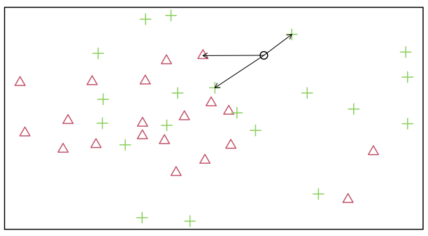
In the simple example in Figure 1 where the black point is to be classified, with \(k=1\) we assign to the green class, with \(k=2\) we assign to the red class (ties being broken in favour of the red class), and with \(k=3\) we assign to the green class.
The choice of \(k\) will clearly have a huge impact on the performance of the classifier. It is often chosen using cross-validation so that, over many splits of the data set into test set and training set, we choose the value of \(k\) that gives the most accurate predictions over all points.
Our main finding is that it is often possible to achieve better performance when the value of \(k\) is allowed to depend on the location of the test point. Indeed, for some constant \(B\) (which may be chosen by cross-validation), when \(n\) is the sample size, \(\bar{f}\) is the marginal density of the data points, and \(x\) is the test point, we find that a choice of \(k\) roughly equal to \[\begin{equation} \tag{1} B \{ n\bar{f}(x) \}^{4/(d+4)} \end{equation}\] results in minimax rate-optimal performance over suitable classes of data-generating mechanisms. In contrast, for heavy-tailed data we see that the standard, fixed-\(k\) classifier is suboptimal. Although \(\bar{f}\) is usually unknown, it can typically be estimated well enough from data. In fact, in many modern applications we have access to large amount of unlabelled \(X\) data that can be used for this purpose.
Theoretical results
Given full knowledge using knowledge of the underlying data-generating mechanism, the optimal decision rule is the Bayes classifier, which assigns points to the class with largest posterior probability. As even this optimal classifier makes mistakes, we typically evaluate the performance of a data-driven classification rule by comparing it to the Bayes classifier. Given a classification rule \(C:\mathbb{R}^d \rightarrow \{0,1\}\), define its excess risk to be \[ \mathcal{E}_P(C)= \mathbb{P}_P\{C(X) \neq Y\} - \mathbb{P}_P\{C^\mathrm{B}(X) \neq Y\}, \] where \(C^\mathrm{B}\) is the Bayes classifier, \(X\) is the test point and \(Y\) is its true class label such that \((X,Y)\) has distribution \(P\). This quantity is non-negative and equal to zero if and only if \(C\) is optimal. Classifiers that make similar predictions to the Bayes classifier perform well.
Our results hold over classes \(\mathcal{P}_{d,\rho}\) of distributions of \((X,Y)\) on \(\mathbb{R}^d \times \{0,1\}\) satisfying certain regularity conditions, including that they have twice-differentiable densities and a bounded \(\rho\)th moment. Ignoring sub-polynomial factors, we find that the standard fixed-\(k\) nearest neighbour classifier, trained on a data set of size \(n\), satisfies \[ \sup_{P \in \mathcal{P}_{d,\rho}} \mathcal{E}_P(C_n^{k\text{nn}}) = O\biggl( \frac{1}{k} + \Bigl( \frac{k}{n} \Bigr)^{\min(4/d,\,\rho/(\rho+d))} \biggr). \] When \(k\) is chosen to minimise this right-hand side, we obtain a rate of convergence of \(n^{-\min(\frac{\rho}{2\rho+d},\frac{4}{4+d})}\).
On the other hand, we find that when \(k\) is chosen according to \((1)\) above, we have \[ \sup_{P \in \mathcal{P}_{d,\rho}} \mathcal{E}_P(C_n^{k_\mathrm{O}\text{nn}}) =O( n^{-\min(\rho/(\rho+d),4/(4+d))}). \] For small values of \(\rho\), i.e. for heavy-tailed distributions, there is a gap between these rates.
Simulation
To illustrate the potential benefits of the local procedure, consider the following simulation. Following Cannings, Berrett and Samworth (2020), we take \(n_1=n_0=100\), \[ P_1 = t_5 \times t_5 \quad \text{ and } P_0 = N(1,1) \times t_5, \] where \(t_5\) is the \(t\)-distribution with \(5\) degrees of freedom. This represents a setting in which there is a gap between the rates of convergence given above. Our results show that the optimal rate here is approximately \(n^{-2/3}\), which is achieved by the local classifier, while with an optimal choice of \(k\) the standard classifier is only guaranteed to achieve a rate of \(n^{-5/12}\).
The data is displayed in the left-most plot of Figure 2, together with vertical lines indicating the action of Bayes classifier, which selects class 0 when the data points lie between the two lines and selects class 1 otherwise. First, we run the standard \(k\)-nearest neighbour classifier on the data, with the value of \(k\) chosen by leave-one-out cross-validation from \(\{1,\ldots,20\}\). The middle plot of Figure shows those points of the data set for which the standard classifier classifies differently to the Bayes classifier. Finally, we run our local classifier, where we assume that \(\bar{f}\) is known, and where the value of \(B\) is chosen by leave-one-out cross-validation on a grid of size \(20\).
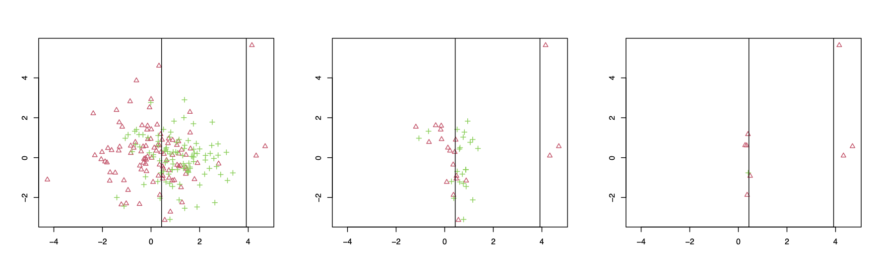 Figure 2. Simulated data and different classifiers.
Perhaps the most striking aspect of the results is that the local classifier agrees with the Bayes classifier much more often than the standard classifier, with only \(9\) disagreements compared to the \(43\) disagreements of the standard classifier. Looking a little closer, we can see that the remaining mistakes that the local classifier makes are concentrated around the Bayes decision boundaries. Standard theoretical analysis of classification problems reveals that such points typically represent the hardest point to classify. We finally see that many, though by no means all, of the points at which the standard classifier makes a mistake appear in low-density regions, for example towards the bottom of the plots.
About the authors
This post was written by Thomas B. Berrett, and was based on
Cannings, T. I., Berrett, T. B. and Samworth, R. J. (2020) Local nearest neighbour classification with applications to semi-supervised learning. Annals of Statistics, 48, 1789–1814. .pdf.
 Timothy I. Cannings is a lecturer in statistics and data science at the School of Mathematics, University of Edinburgh. He completed his PhD with Prof Richard Samworth in the Statistical Laboratory at the University of Cambridge in 2015. He then worked with Prof Yingying Fan as a Postdoc at the University of Southern California.
 Thomas B. Berrett is an Assistant Professor in the Department of Statistics at the University of Warwick. He completed his PhD with Prof Richard Samworth in the Statistical Laboratory at the University of Cambridge in 2018, and later worked as a Postdoc with Prof Cristina Butucea at CREST, ENSAE, Institut Polytechnique de Paris.
 Richard J. Samworth is Professor of Statistical Science and Director of the Statistical Laboratory at the University of Cambridge. He is also a Teaching Fellow at St John’s College.