We look at the problem of learning latent structure between two blocks of data through the partial least squares (PLS) approach. These methods include approaches for supervised and unsupervised statistical learning. We review these methods and present approaches to decrease the computation time and scale the method to big data
Given two blocks of data, the PLS approach seeks latent variables which are constructed as linear combinations of the original datasets. These latent variables are constructed according to specific covariance or correlation requirements. As such the latent variables can be used as a data reduction tool that sheds light on the relationship between the datasets. For two blocks of data there are four established PLS methods that can be used to construct these latent variables:
- PLS-SVD
- PLS-W2A
- Canonical correlation analysis (CCA)
- PLS-R
These methods provide a range of useful methods for data exploration and prediction for datasets with high dimensional structure. However, as shown in the sparse PCA literature (Johnstone 2004) in high dimensional settings (\(n<<p\)) the standard latent variable estimates may be biased and sparsity inducing methods are a natural choice. After reviewing the two-block PLS methods and placing them in a common framework we provide details for the application of sparse PLS methods that use regularisation via either the lasso or sparse group lasso penalisation.
Finding the latent variables
Let \(X: n\times p\) and \(Y: n\times q\) be the datasets comprised of n observations on p and q variables respectively, the latent variables \(\xi = X u\) and \(\omega = Y v\) bare a striking similarity to the principal components from principal component analysis (PCA) where \(u\) is a p-vector and \(v\) is a q-vector. The PLS-SVD, PLS-W2A and PLS-R methods optimise the sample covariance between the latent variables \[ \text{max}_{\xi,\omega} \widehat{Cov}(\xi, \omega) \rightarrow \text{max}_{u,v} \widehat{Cov}(Xu, Yv) = \text{max}_{u,v} u^TX^TYv \] subject to \(\|u\|=\|v\| = 1\) and orthogonality constraints for the different methods. Whereas CCA optimises \[ \text{max}_{\xi,\omega} \widehat{Corr}(\xi, \omega) \rightarrow\text{max}_{u,v} \widehat{Corr}(Xu, Yv) = \text{max}_{u,v} u^T(X^TX)^{-1/2}X^TY(Y^TY)^{-1/2}v \] subject to orthogonality constraints similar to the PLS-SVD. These orthogonality constraints are enforced by removing the effect of the constructed latent variables using projection matrices. Once the effect has been removed the optimisation is repeated on the projected data. This process is the same for all PLS methods and can be simply adjusted to allow for sparsity in the weights (\(u\) and \(v\)) using sparse regularising penalties (e.g. lasso, group lasso, sparse group lasso).
Computational speedups
Due to the algorithmic similarity of the different methods some additional computational approaches can be used to speed up the required computation for the PLS approach. In our paper, we consider reducing memory requirements and speeding up computation by making use of the “bigmemory” R package to allocate shared memory and make use of memory-mapped files. Rather than loading the full matrices when computing the matrix cross-product (\(X^TY\), \(X^TX\) or \(Y^TY\)) we instead read chucks of the matrices, compute the cross-product on these chucks in parallel, and add these cross-products together, ie. \[ X^TY = \sum_{c=1}^CX_c^TY_c \] where \(X_c\) and \(Y_c\) are matrix chucks formed as the subsets of the rows of \(X\) and \(Y\). Additional computational approaches are used for when either p or q are large or when n is very large and data is streaming in while q is small.
Example on EMNIST
We show an example using PLS regression for a discrimination task, namely the extended MNIST dataset. This data set consists of n = 280,000 handwritten digit images. It contains an equal number of samples for each digit class (0 to 9) where the dimension of the predictors is \(p=784\) with \(q=10\) classes. The images are already split into a training set of 240,000 cases and a test set of 40,000 cases. Since we have a large sample size \(n > p, q\) we opt not to consider regularisation for this example. The PLS-DA method is able to recover an accuracy of 86% in around 3 minutes using 20 latent variables and 2 cores.

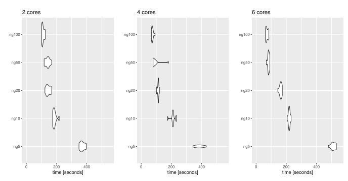
We investigated the relationship between the number of chunks and the number of cores used in the algorithm. The plot below shows the elapsed computation time for fitting a single component of the PLS discriminant analysis algorithm using 2, 4 or 6 cores (on a laptop equipped with 8 cores). On the vertical axis, \(ngx\) indicates that \(x\) chunks were used in our algorithm.