Abstract
Co-clustering techniques, which group observations and features simultaneously, have proven to be efficient in summarising data sets. They exploit the dualism between rows and columns and the data set is summarized in blocks (the crossing of a row-cluster and a column-cluster). However, in the case of mixed data sets (with features of different kind), it is not easy to define a co-clustering method that takes this heterogeneity into account. For this purpose, we present how to use the Multiple Latent Block Model (Robert 2017) on mixed data.
Multiple Latent Block Model for mixed data
The Multiple Latent Block Model (MLBM) is an extension the Latent Block Model (LBM) (Nadif and Govaert 2008), which is a probabilistic approach to perform co-clustering. It consists in separating the data matrix in \(D\) matrices \(\boldsymbol{x}^{(d)}\) such that \(D\) is the number of kinds of data. For the sake of simplicity, we consider here that \(\boldsymbol{x}\) has two different kinds of features (i.e \(D=2\)). The MLBM performs a co-clustering such that the row-clusters partition is the same for all \(\boldsymbol{x}^{(d)}\), and that there is a column-clusters partition for every \(\boldsymbol{x}^{(d)}\).

Example of a mixed-data matrix with two different kinds of features co-clustered with the MLBM.
Notations
We consider that the data matrix \(\boldsymbol{x}\) has two different kinds of features, we note:
- the data matrix \(\boldsymbol{x}=(\boldsymbol{x}^{(1)},\boldsymbol{x}^{(2)})\), and we will refer to \(\boldsymbol{x}^{(d)}\) in the general case (with \(d \in \{1,2\}\)),
- \(N\) rows, \(J_1\) columns for \(\boldsymbol{x}^{(1)}\) and \(J_2\) columns for \(\boldsymbol{x}^{(2)}\),
- \(G\) row-clusters, \(H_1\) column-clusters for \(\boldsymbol{x}^{(1)}\) and \(H_2\) column-clusters for \(\boldsymbol{x}^{(2)}\),
- the latent variables of the model \(\boldsymbol{v},\boldsymbol{w}=(\boldsymbol{v},\boldsymbol{w}^{(1)},\boldsymbol{w}^{(2)})\):
- \(\boldsymbol{v}\) is the row partition matrix of size \((N \times G)\) that indicates the cluster assignments, i.e \(\boldsymbol{v}_i = (v_{i1},\ldots,v_{iG})\) with \(v_{ig}=1\) when observation \(i\) belongs to row cluster \(g\) and \(v_{ig}=0\) otherwise.
- \(\boldsymbol{w}^{(d)}\) is the column partition matrix of size \((J_d \times H_d)\) that indicates the cluster assignments, i.e \(\boldsymbol{w}^{(d)}_j = (w_{j1},\ldots,w_{jH_d})\) with \(w_{jh}^{(d)}=1\) when feature \(j\) belongs to column cluster \(h\) and \(w_{jh}^{(d)}=0\) otherwise,
- a block refers to the crossing of a row-cluster and of a column-cluster.
Finally, for better readability, we sometimes highlight:
- the latent variable and parameters that relate to row-clusters in blue (e.g \(\boldsymbol{v}= \color{blue}{\boldsymbol{v}}\)),
- the latent variable and parameters that relate to column-clusters in green (e.g \(\boldsymbol{w}= \color{ForestGreen}{\boldsymbol{w}}\)),
- the parameters that relate to blocks in red (e.g \(\boldsymbol{\alpha}_{gh}= \color{red}{\boldsymbol{\alpha}_{gh}}\)).
Assumptions
The MLBM relies on several assumptions. The first one states that the \(2\) data matrices are conditionally independent of the row and column partitions:
\[ p(\boldsymbol{x}|\boldsymbol{v},\boldsymbol{w}) = p(\boldsymbol{x}^{(1)}|\boldsymbol{v},\boldsymbol{w}^{(1)}) \times p(\boldsymbol{x}^{(2)}|\boldsymbol{v},\boldsymbol{w}^{(2)}) \].
In addition, the univariate random variables \(x_{ij}^{(d)}\) are assumed to be conditionally independent on partitions \(\boldsymbol{v}\) and \(\boldsymbol{w}^{(d)}\). Thus, the conditional probability function of \(\boldsymbol{x}\) given \(\boldsymbol{v}\) and \((\boldsymbol{w}^{(d)})_d\) is expressed as:
\[ p(\boldsymbol{x}|\boldsymbol{v},\boldsymbol{w};\boldsymbol{\alpha}) = \underset{i,j,g,h}{\prod} p(x_{ij}^{(1)}; \alpha_{gh}^{(1)})^{v_{ig}w_{jh}^{(1)}} p(x_{ij}^{(2)}; \alpha_{gh}^{(2)})^{v_{ig}w_{jh}^{(2)}}, \]
where \(\boldsymbol{\alpha}=(\boldsymbol{\alpha}^{(d)})_d\) with \(\boldsymbol{\alpha}^d=(\alpha_{gh}^{(d)})_{g,h}\) is the distribution parameters of block \((g,h)\) of matrix \(\boldsymbol{x}^{(d)}\). It depends on the distribution one uses to model the data. For instance, in the case of the Gaussian distribution, \(\alpha_{gh}^{(d)} = (\boldsymbol{\mu}^{(d)}_{gh}, \boldsymbol{\Sigma}^{(d)}_{gh})\). Let us note too that the chosen distributions can be different for each kind of data.
Second, the latent variables \(\boldsymbol{v},\boldsymbol{w}^{(1)},\boldsymbol{w}^{(2)}\) are assumed to be independent, so: \(p(\boldsymbol{v},\boldsymbol{w};\boldsymbol{\gamma},\boldsymbol{\rho}) = p(\boldsymbol{v};\boldsymbol{\gamma})p(\boldsymbol{w}^{(1)};\boldsymbol{\rho}^{(1)})p(\boldsymbol{w}^{(2)};\boldsymbol{\rho}^{(2)})\), where:
\[ p(\boldsymbol{v};\boldsymbol{\pi}) = \underset{i,g}{\prod}\pi_g^{v_{ig}} \] and
\[ p(\boldsymbol{w}^{(d)};\boldsymbol{\rho}^{(d)}) = \underset{j,h}{\prod}{\rho_h^{(d)}}^{w_{jh}^{(d)}} \].
So, if \(V\) and \((W^{(d)})_d\) are the sets of all possible partitions \(\boldsymbol{v}\) and \((\boldsymbol{w}^{(d)})_d\), the probability density function \(p(\boldsymbol{x}; \boldsymbol{\theta})\) is written: \[ p(\boldsymbol{x};\boldsymbol{\theta})= \underset{(\color{blue}{\boldsymbol{v}},\color{ForestGreen}{\boldsymbol{w}^{(1)}},\color{ForestGreen}{\boldsymbol{w}^{(2)}})\in V\times W^{(1)} \times W^{(2)}}{\sum} \underset{i,g}{\prod}\color{blue}{\pi_g^{v_{ig}}} \underset{j,h}{\prod}\color{ForestGreen}{{\rho^{(1)}_h}^{w_{jh}^{(d)}}} \underset{i,j,g,h}{\prod}p(x_{ij}^{(1)}; \color{red}{\alpha_{gh}^{(1)}})^{\color{red}{v_{ig}w_{jh}^{(1)}}} \underset{j,h}{\prod}\color{ForestGreen}{{\rho^{(2)}_h}^{w_{jh}^{(2)}}} \underset{i,j,g,h}{\prod}p(x_{ij}^{(2)}; \color{red}{\alpha_{gh}^{(2)}})^{\color{red}{v_{ig}w_{jh}^{(2)}}}. \]
Generative process
The generative process of a cell \(x^{(d)}_{ij}\) of the matrix is as follows: \[ \begin{align*} &\color{blue}{\boldsymbol{v}_i} \sim \mathcal{M}(1,\color{blue}{\boldsymbol{\pi}}), \\ &\color{ForestGreen}{\boldsymbol{w}^{(d)}_j} \sim \mathcal{M}(1,\color{ForestGreen}{\boldsymbol{\rho^{(d)}}}), \\ &x_{ij}^{(d)} | \color{red}{v_{ig}=1, w_{jh}^{(d)}=1} \sim f(x_{ij}^{(d)};\color{red}{\boldsymbol{\alpha}^{(d)}_{gh}}). \end{align*} \]
Inference of the model
Once we defined the generative process of a data set, the goal is to estimate the parameters \(\boldsymbol{\theta}\) of this generative process according to the data, and also to deduce the latent variables from them. In this case, we need to compute \(\boldsymbol{\theta}=(\color{blue}{\boldsymbol{\pi}}, \color{ForestGreen}{\boldsymbol{\rho}^{(1)}}, \color{ForestGreen}{\boldsymbol{\rho}^{(2)}}, \color{red}{\boldsymbol{\alpha}^{(1)}_{gh}}, \color{red}{\boldsymbol{\alpha}^{(2)}_{gh}})\), and to deduce the row partitions \(\color{blue}{\boldsymbol{v}}\) and column partitions \((\color{ForestGreen}{\boldsymbol{w}^{(1)}},\color{ForestGreen}{\boldsymbol{w}^{(2)}})\). In the Maximum Likelihood Estimation framework, the Expectation-Maximisation (EM) algorithm is often used in such contexts with parameters and latent variables to be estimated. Unfortunately, the Expectation step is not tractable because it requires the calculation of many terms, which is not feasible in a reasonable amount of time. The Multiple Latent Block Model and more generally the methods based on the Latent Block Model use variants of the EM-algorithm such as the Stochastic-EM-Gibbs algorithm.
Use-case: analysing a health quality survey in oncology
The data set that motivated this work is a psychological survey on women affected by a breast tumour. Patients replied at different stages of their treatment to questionnaires with answers on ordinal scales. The questions relate to different aspects of their life referred to as “dimensions.” In this use-case, we focus on three different dimensions: anxiety, depression and symptoms. The questions that relate to these dimensions are considered to be of different kinds because they are not necessarily on the same ordinal scale. In addition, they are seen as different in a semantic way by the pychologists since they do not refer to the same dimensions. The figure below represents the data set: the women are projected onto rows and the questions are projected onto columns. Therefore, the cell \((i, j)\) is the response of patient \(i\) to question \(j\). The shades of grey indicate how positively the individual replied. For instance, for the question “Have you had trouble sleeping?” if the patient answers “Not at all,” the corresponding cell will be white, whereas a response such as “Very much” will correspond to a black cell.
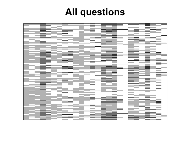
Questionnaire’s graphical representation: patients are projected onto rows and questions are projected onto columns.
As explained previously, the MLBM separates the features that are considered as different, and simultaneously performs a clustering on the rows and a clustering on the columns of each isolated matrix. The figure below shows the result for our use-case. We note \(5\) row-clusters, i.e. \(5\) patients profiles. Furthermore, the column-clusters helps summarising these profiles: by grouping the questions that have the same behaviour with respect to the row-clusters it is easier to distinguish the differences between these profiles.
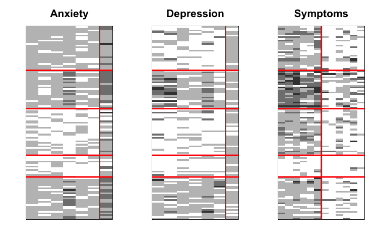
Questionnaire co-clustered with the MLBM.
Remarks
This blog post is based on (Selosse, Jacques, and Biernacki 2020) and (Selosse et al. 2019). Furthermore, The R package mixedClust implements the Multiple Latent Block Model and will be available on the CRAN soon.
About the authors:
 Margot Selosse received her Ph.D. degree from Université Lumière Lyon II in 2020. She currently is a post-doctoral researcher in the Thoth team at Inria grenoble. Her main research area is related to clustering, mixed-type data and graph representation learning.
 Julien Jacques received his Ph.D. degree in applied mathematics from University of Grenoble, France. In 2006 he joined University of Lille where he held the position of Associate Professor. In 2014, he joined University of Lyon as Full Professor in Statistics. His current research in statistical learning concerns the design of clustering algorithm for functional data, ordinal data and mixed-type data. He is a member of the French Society of Statistics.
- Christophe Biernacki is a Scientific Deputy at Inria Lille and Scientific Head of the Inria MODAL research team, and received his Ph.D. degree from Université de Compiègne in 1997. His research interests are focused on model-based and model-free clustering of heterogeneous data.