Introduction

New statistical process control (SPC) methods have to be developed in order to handle more and more complex data, which are available because of the advent of new data acquisition technologies. In particular, in many practical situations the quality characteristic of a process can be modelled as a function defined on a compact domain, data of such kind are the foundation of a rapidly expanding area of statistics referred to as functional data analysis (FDA). SPC methods which allow monitoring and controlling such processes are known as profile monitoring techniques. As in the classical SPC (i.e., where data are scalars) profile monitoring control charts have the task of continuously monitoring the quality characteristic and of triggering a signal when assignable sources of variations (i.e., special causes) act on it. When this happens, the process is said to be out-of-control (OC). On the contrary, the process is said to be in-control (IC) when only normal sources of variation (i.e., common causes) apply.

Often, measures of other functional covariates related to the quality characteristic are available. To this end, we propose a new control chart that continuously monitors the quality characteristic using information coming from the other functional covariates. The idea is to adjust the quality characteristic value in order to improve the accuracy and the effectiveness of the chart in identifying assignable sources of variations acting on the process. This chart is referred to as functional regression control chart (FRCC) due to the similarity to the regression control chart, which arises in the multivariate (non functional) context. The proposed methodology is implemented in the R package funcharts available at https://github.com/unina-sfere/funcharts.

The Functional Regression Control Chart Framework

The FRCC can be regarded as a general framework for profile monitoring that can be divided into three main steps. Firstly, (i) define a functional regression model to be fitted $$\label{eq_generalmodel} \tilde{Y}=g\left(\mathbf{\tilde{X}}\right)+\varepsilon,$$ where $\tilde{Y}$ is the functional response variable, which represents the functional quality characteristic, and $\varepsilon$ is a functional error term, both defined on the compact domain $\mathcal{T}$, $g$ is a generic function of a vector $\mathbf{\tilde{X}}$ of random functional covariates $\tilde{X}_1,\dots,\tilde{X}_p$, defined on the compact domain $\mathcal{S}$. Secondly, (ii) define the estimation method of the chosen model, and, thirdly (iii) define the monitoring strategy of the functional residual defined as $$\label{eq_generalresiduals} \tilde{e}=\tilde{Y}-\widehat{\tilde{Y}} ,$$ where $\widehat{\tilde{Y}}$ is the fitted value of $\tilde{Y}$.

In particular, to obtain a specific implementation of the FRCC, we assume that the covariates $\mathbf{X}$ linearly influence the response $Y$ through the multivariate functional linear regression model, that is $$\label{eq_lm} Y\left(t\right)=\int_{\mathcal{S}}\left(\mathbf{\beta}\left(s,t\right)\right)^{T}\mathbf{X}\left(s\right)ds+\varepsilon\left(t\right)\quad t \in \mathcal{T},$$ where $Y$ and $\mathbf{X}$ are the standardized versions of $\tilde{Y}$ and $\tilde{\mathbf{X}}$, and $\mathbf{\beta}=\left(\beta_1,\dots,\beta_p\right)^{T}$ is the coefficient vector. An estimator $\hat{\mathbf{\beta}}$ of the coefficient vector $\mathbf{\beta}$ is obtained using $n$ i.i.d. observations of the response and predictor variables, and considering the *multivariate functional principal component* or Karhunen–Loève decomposition of $Y$ and $\mathbf{X}$. To monitor the residual $\tilde e$, we consider the Hotelling’s $T^{2}$ and the squared prediction error ($SPE$) control charts based on the scores of the functional principal component decomposition. The control limits are calculated using percentiles of the empirical distributions of the two statistics, estimated considering observations acquired under in-control conditions and an overall Type I error. This phase, along with the estimation of $\mathbf{\beta}$, will be referred to as Phase I. For a new observation, the residual and, thus, the $T^{2}$ and $SPE$ statistics are calculated and an alarm signal is issued if at least one statistic violets the control limits (Phase II).

Real-case Study: Fuel Consumption Monitoring in the Shipping Industry

To demonstrate the potential and the applicability of the proposed control chart in practical situations, a real-case study in the shipping industry is presented. It addresses the issue of monitoring ship fuel consumption and, thus, $\text{CO}_{\text{2}}$ emissions, which, in view of the dramatic climate change, is of great interest in the maritime field in the very last years. In particular, real data are collected from a Ro-Pax ship owned by the Italian shipping company Grimaldi Group linking two ports in the Mediterranean sea from December 2014 to October 2017. The following figure shows the 315 profiles observed for the covariates and response.

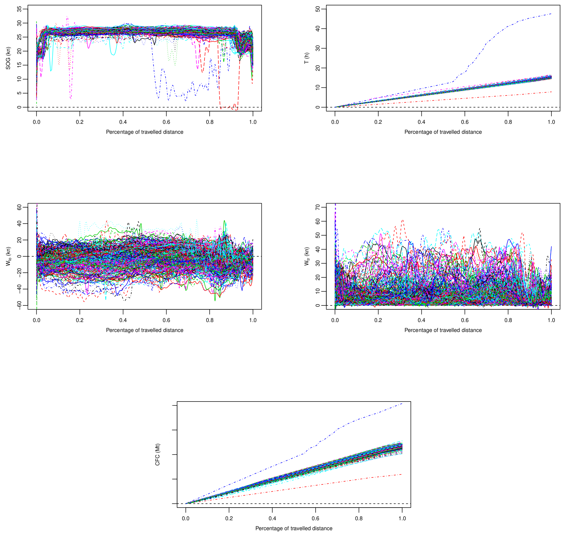
In particular, the cumulative fuel consumption ($CFC$) per each voyage is considered as the response variable, whereas, the sailing time ($T$), measured in hours ($h$), the speed over ground ($SOG$), measured in knots ($kn$), and the longitudinal and transverse wind components ($W_{lo}$ and $W_{tr}$), measured in knots ($kn$), are assumed as the predictors.

During February 2016 energy efficiency operations were performed that produced a shift in the response mean. In light of this, observations before energy efficiency operations are used in Phase I, whereas the remaining observations are used to perform Phase II. To evaluate the FRCC performance, two competitor profile monitoring schemes are considered. They consist of monitoring scores coming from a principal decomposition of the response by means of Hotelling’s $T^{2}$ and the $SPE$ control charts (hereafter denoted as RESP control chart), and of monitoring the area under the response curve (hereafter denoted as INBA control chart). The performance of the three charts is evaluated by means of the average run length ($\text{ARL}$).

In the following figure, each observation is plotted onto the FRCC control chart and the two competitor ones.

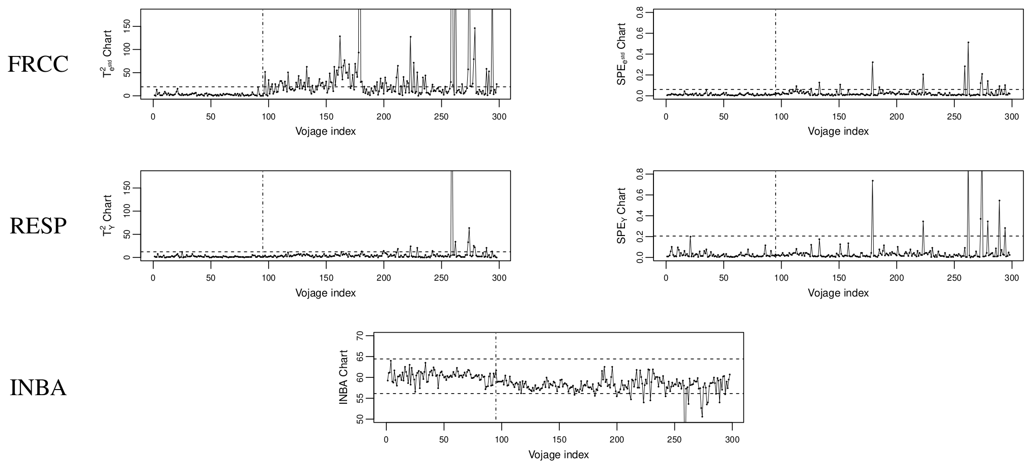
By comparing the three charts, the responsiveness of the FRCC is evidently higher than that of the the INBA and the RESP control charts which signal a much lower number of OCs. In particular, for the FRCC the change in the response mean is almost exclusively captured by the $T^{2}$ control chart, which means that dissimilarities between the Phase I and Phase II samples occur mostly in the space spanned by the retained principal components. Moreover, by looking at the following table, the estimated $\text{ARL}$ ($\widehat{\text{ARL}}$) achieved by FRCC is at least a fourth of those achieved by the RESP and INBA control charts. This further confirms that the FRCC outperforms the competitor control charts.

This article is based on
Centofanti, Fabio, Antonio Lepore, Alessandra Menafoglio, Biagio Palumbo, and Simone Vantini. "Functional Regression Control Chart." Technometrics (2020): 1-14, DOI: https://doi.org/10.1080/00401706.2020.1753581.

Authors’ biography

Fabio Centofanti is a PhD student at the Department of Industrial Engineering of the University of Naples Federico II, Italy, fabio.centofanti@unina.it. His research interests include functional data analysis and statistical process monitoring.

Antonio Lepore is an Assistant Professor at the Department of Industrial Engineering of the University of Naples Federico II, Italy, antonio.lepore@unina.it. His main research interests include the industrial application of statistical techniques to the monitoring of complex measurement profiles from multi-sensor acquisition systems, with particular attention to renewable energy and harmful emissions.

Alessandra Menafoglio is an Assistant Professor at MOX, Department of Mathematics, Politecnico di Milano, alessandra.menafoglio@polimi.it. Her research interests focus on the development of innovative statistical models and methods for the analysis and statistical process control of complex observations (e.g., curves, images, functional signals), possibly characterized by spatial dependence.

Biagio Palumbo is an Associate Professor in “Statistics for experimental and technological research” at the Department of Industrial Engineering of the University of Naples Federico II, Italy, biagio.palumbo@unina.it. His major research interests include reliability, design and analysis of experiments, statistical methods for process monitoring and optimization and data science for technology.

Simone Vantini is Associate Professor of Statistics at the Politecnico di Milano, Italy, simone.vantini@polimi.it. He has been publishing widely in Functional and Object-Oriented Data Analysis. His current research interests include: permutation testing, nonparametric forecasting, process control, non-Euclidean data, and in general statistical methods and applications motivated by business or industrial problems.